Complexity
Polynomial versus exponential algorithms
Suppose we have two algorithms, one with running time n2 seconds and one with running time 2n seconds. Let's compare how long it takes them to run for a few values of n.
| n | n2 | 2n |
| 5 | 25 | 32 |
| 10 | 100 | 1024 |
| 20 | 400 | 1048576 |
| 30 | 900 | 1073741824 |
| 40 | 1600 | 1099511627776 |
| 50 | 2500 | 1125899906842624 |
Generally, a polynomial-time algorithm is anything whose big O running time is nk or better for some integer k. For instance, O(n), O(n2), O(n3), and O(n4) are all polynomial time, as are O(1), O( log n), O(n log n), and O(n3.14), as those are all at least as good as polynomial time algorithms. If a problem has a polynomial-time algorithm, then there is good chance that the algorithm solves the specific instances of the problem we care about in a reasonable amount of time. But if all we have is an exponential or worse algorithm, then most likely we won't be able to solve the problem in a reasonable amount of time except when n is very small.
Complexity classes
Computer scientists divide up problems into various classes. P is the name of the class of problems that can be solved with polynomial time algorithms. Most problems you run into in early programming classes are in P. These are things like summing the items in a list of integers, finding the largest thing in a list, counting how many things in a 2d array are equal to 0, etc. P also includes the problems of searching for an item in a list, finding shortest paths in graphs, and finding minimum spanning trees.
The preceding paragraph is a little inaccurate. The way computer scientists define P, it only consists of decision problems. These are problems for which the answer is always yes or no. For instance, determining if a list contains a certain element is a decision problem since it has a yes/no answer, but finding the index of that element is not a decision problem. Likewise, determining if a graph has a shortest path of cost 20 or less is a decision problem, while finding the cheapest cost of a path is not. That problem is actually an optimization problem. There are techniques for turning optimization problems into decision problems. For instance, the shortest path decision problem can be used to find the length of the shortest path by asking if there is a path of cost 1, if there is a path of cost 2, if there is a path of cost 3, etc. Decision problems are a little easier to analyze than optimization problems, and since optimization problems can be turned into decision problems, the definition of P just involves decision problems.
The second important complexity class we will cover is called NP. The name is short for “nondeterministic polynomial time”. Specifically, it has to do with a decision problem being solvable in polynomial time by a nondeterministic Turing machine, but that definition is tricky. An easier way to think about NP is that it's the class of decision problems where if we are given a solution to a problem, then we can verify that the solution is correct in polynomial time. We may or may not be able to solve the problem in polynomial time, but we can check if the solution is correct in polynomial time.
Here is an example. It's called the subset sum problem. The problem is very simple: given a set of numbers, determine if there is a subset of them that adds up to 0. For instance, below is a set of numbers. See if you can find a subset of them that adds up to 0.
 If you tried it, you probably found that it took some time to find a solution. The simplest solution I know of is {–43, 3, 4, 36}. But, once we have a solution, it's very easy to check that it works—just add up all the numbers and see if you get 0. For this example, –43+3+4+36 = 0, so it works. From this problem remember this: it is tricky to find a solution, but if we are given a solution, then it is easy to check that it works.
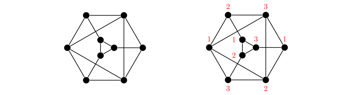
Here is another example. In graph coloring, we are trying to assign numbers (traditionally called colors) to the vertices of a graph so that adjacent vertices get different colors. Try to find a coloring of the graph on the left using 3 colors. It will take some time. But it's quick to verify that the graph on the right uses 3 colors and satisfies the rule of neighbors getting different colors. I teach graph coloring in several classes, and I can grade a graph coloring problem in a few seconds, while it typically takes people a few minutes to solve it.
One final example is Sudoku puzzles. A tricky Sudoku puzzle can take a half hour or more to solve, but it only takes a minute to check that a solution is valid.
The basic idea of NP problems is that given a solution, it is easy (i.e. takes polynomial time) to verify that the solution works. NP problems may or may not be hard to solve, but they always have the property that if someone gives us a solution, then we can easily check if it works.
The P=NP problem
This brings us to the most famous problem in all of computer science: the P=NP problem. It asks if the classes P and NP are the same. Thinking of polynomial-time problems as easy, at least in comparison to exponential problems, we can think of the P=NP problem as asking the following:
If it is easy to check that a solution to a problem works, must that mean that it is also easy to solve the problem?
Based on the examples just given, it would seem like the answer is clearly no. Most mathematicians and computer scientists think the answer is no, but no one can prove it. The P=NP problem has a million-dollar prize attached to it, and it is arguably the most famous unsolved problem in all of computer science. If someone were to prove that P ≠ NP, probably nothing much would change in the world of computer science other than that person becoming very famous. But if someone were to actually show that P = NP, that would likely completely upend all of computer science. Everything that we thought was hard would end up being easy. It's a little like how practical quantum computers will one day break most of modern cryptography, except that showing P = NP would not only break that but everything else as well.
Complexity classes
As we have seen, P consists of problems that are solvable in polynomial time. NP consists of problems where if we are given a solution, we can check that it's correct in a polynomial amount of time. P is a subset of NP because for any problem in P, if we are given a solution to it, we can check that it works in polynomial time by just re-solving the problem ourselves. Since the problem is in P, that re-solving process will take a polynomial amount of time.
Let's introduce a new class called NP-hard. It is defined to be those problems that are at least as hard as any problem in NP. Specifically, if A is an NP-hard problem and we could find a polynomial time solution to A, then we could use that solution to find a polynomial time solution to any problem in NP. Because of the “at least” in the definition, NP-hard problems include some problems in NP and some problems that are more difficult than anything in NP. The NP-hard problems that are in NP are called NP-complete. This Venn diagram shows the relationship between all these classes, assuming P ≠ NP.

Looking at the various regions of the diagram, we think of the P region as “easy” problems. The part of NP-hard that is outside of NP, the rightmost area in the picture, consists of “really hard” problems. The NP region contains some “easy” problems (those in P), and some problems that seem to be hard, like the subset sum problem and n × n Sudoku puzzles.
A very important part of this picture is the NP-complete area, which is covered in the next section. An interesting, but not well-understood, part of the diagram is the part of NP that lies outside of the P and NP-complete regions. Only a few problems of practical interest are in this region. One of those is integer factorization. It seems to be a hard problem, but no one knows for sure. The fact that it seems to be hard is the basis for RSA encryption, which is important in internet security. If someone were to find a practical algorithm for factoring large integers, it would cause a lot of problems for internet security.
NP-complete problems
There are a huge number of important problems in the NP-complete class. They are all difficult in that no one has found algorithms better than exponential for them. Over 1000 problems have been identified as NP-complete. Here is a list of some important ones:
- Subset sum problem — Given a set of integers, determine if some subset adds up to 0.
- Graph coloring — Given a graph G and an integer k, determine if the vertices of G can be colored with k colors so that neighbors never get the same color.
- Hamiltonian cycle — Given a graph, determine if there is a path that starts and ends at the same vertex and goes through each vertex exactly once. A Hamiltonian cycle is highlighted below on the left.
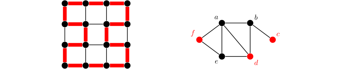
- Independent set — Given a graph and an integer k, does the graph have an independent set of size k? An independent set is a set of vertices none of which are neighbors of each other. The set {c, d, f} highlighted in the graph above on the right is an independent set.
- Knapsack problem — Given a list of prices and weights of items that we want to put into a knapsack, if the knapsack has a given weight limit, can we obtain a total price of some desired amount?
The problems above all have a ton of applications to real-world problems including to things like scheduling, routing, and biology. There are also many game problems that are NP-complete including n × n Sudoku, Freecell, and Super Mario Brothers. One of the things that makes NP-complete problems so important is that based on the definition of NP-hard and NP-complete, if you could find a polynomial-time solution for even one of these problems, then you could use that to find a polynomial-time solution for every one of the NP-complete problems.
It is also interesting that small changes to the problem statements can make the difference between a problem in P and an NP-complete problem. For instance,
- Finding the shortest path in a graph is in P.
Finding the longest path in a graph is NP-complete. - Finding a round trip in a graph visiting each edge exactly once is in P (an Eulerian circuit).
Finding a round trip in a graph visiting each vertex exactly once is NP-complete (a Hamiltonian cycle). - Determining if a system of inequalities has a real number solution is in P.
Determining if a system of inequalities has an integer solution is NP-complete. - Determining if a graph can be colored with 2 colors is in P.
Determining if a graph can be colored with 3 colors is NP-complete. - Determining if it is possible to break a group of people into compatible teams of 2 is in P.
Determining if it is possible to break a group of people into compatible teams of 3 is NP-complete.
Showing a problem is NP-complete
There is a famous problem in computer science called satisfiability (SAT for short). It involves logical expressions using ∧ (AND) ∨ (OR), and ~ (NOT). Any expression using these three operations can be rewritten into a special form called conjunctive normal form. In this form, each expression consists of several clauses AND-ed together, where each clause has the same number of variables, and those variables or their negations are all OR-ed together in those clauses. Here are a few examples:


The first example is called a 2-SAT problem because each clause has two variables in it. The second is called 3-SAT because there are three variables in each expression. The goal of satisfiability is to find a set of true and false values for the variables that make the overall expression true. For example, in the first example above, if we set b to false and the other variables to true, then that would make the entire expression true.
Satisfiability is important because a lot of other problems can be rewritten as satisfiability problems, and there are some highly optimized SAT solvers out there. The solution to the SAT problem can then be transformed to give a solution to the original problem.
Satisfiability is also important because 3-SAT was the first problem proved to be NP-complete. Once that had been established, other problems could be showed to be NP-complete by showing that if you could solve them in polynomial time, then you could solve 3-SAT in polynomial time. This leads to a general technique for showing something is NP-complete, called a reduction. There are two steps to showing a problem A is NP-complete:
- First, show A is in NP by giving a polynomial-time algorithm that can be used to verify solutions to A.
- Then pick any problem B already known to be NP-complete (such as 3-SAT), and show how to rewrite it in a polynomial number of steps as an instance of problem A, such that solving problem A would give a solution to problem B.
We will look at a couple of examples here.
First, we need to say why the problem is in NP. That is, if someone gives us a solution, we need to be able to quickly verify if it works. A solution to the independent set problem would be a set of k vertices that are all non-neighbors. To do this, we first need to make sure it has k vertices, which is easy. Then we need to make sure none of those vertices are neighbors. If we store the graph with adjacency lists, then this can be done in polynomial time by looping over the k vertices and seeing if any of the other vertices are in each vertex's list.
Second, to show it is NP-complete, we will use a reduction to 3-SAT. We'll describe the process with an example. Suppose we are given the following 3-SAT problem:
(a ∨ b ∨ c) ∧ (~a ∨ ~b ∨ c) ∧ (a ∨ b ∨ ~c). We can turn it into the graph below.
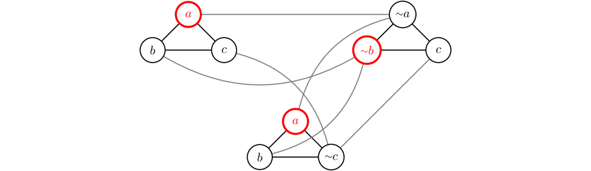
The rules for converting it are as follows:
- For each clause of the 3-SAT program, make a vertex for each variable.
- Add an edge from each vertex of a clause to each other vertex in that same clause.
- Add an edge between each pair of vertices anywhere in the graph that correspond to a variable and its negation.
The purpose of this is to convert the 3-SAT problem into an independent set problem where finding the independent set will give us a solution to the 3-SAT problem. In particular, we are then looking for an independent set of size equal to the total number of clauses. If we can't find such an independent set, then the 3-SAT problem has no solution. In the graph above, an independent set is highlighted. It tells us choose a from the first clause, ~b from the second clause, and a from the third clause. This tells us that setting a to true and b to false will solve the 3-SAT problem. It doesn't tell us anything about c, so we could set it to either true or false. Both would work.
To see why this construction works, note that by adding an edge from each variable to its negation, we guarantee that we can never choose both a variable and its negation when doing an independent set. For instance, if we could choose both a and ~a, that would be saying a is both true and false at the same time, which isn't logically reasonable. By adding edges between every vertex and every other vertex in a clause, we guarantee that we can never take more than one vertex from a clause when doing the independent set. And forcing the independent set to have the same size as the number of clauses forces us to have to pick one vertex from each clause in order to find a solution. With a little more work, we could prove that if there is no independent set of the right size then there is no solution, but we will skip that here.
First, we have to show the problem is in NP. That is, given a solution to the problem, we need to show that in polynomial time we can verify it works. A potential solution is a set of k vertices that are all supposed to be adjacent to each other. Given a potential solution, we can easily check if there are k vertices in it, and checking if they are all neighbors of each other is also quick, being very similar to the independent set problem.
Second, to show that it is NP-complete, we do a reduction to the independent set problem, which we just showed is NP-complete. The trick is to notice that cliques are in some sense the opposite of independent sets. A clique is a set of vertices that are all neighbors, and an independent set is a set of vertices that are all non-neighbors.
So let's say we're given a graph and we are looking for an independent set of size k. We need to show how to use the k-clique problem to find the independent set. Based on the previous paragraph, the trick is to take the complement. The complement of a graph is a graph with the same vertices, where the edges are reversed. Specifically, if there is an edge between two vertices in the original graph, then is is no edge between them in the complement, and if there is no edge between them in the original, then there is an edge between them in the complement. See below for an example:
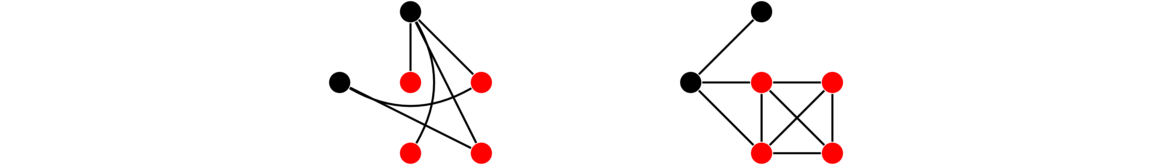
The key idea then is that independent sets in the original correspond to cliques in the complement (and vice-versa). So if the complement has a clique of size k, then the original must have an independent set of size k.
Practical matters
There is a lot to take in from this set of notes. Don't expect to absorb it all on the first read. The basic idea is that there are some problems that can be solved relatively quickly (in polynomial time), and there is a large group of practical problems (NP-complete and NP-hard) for which all we have are slow (exponential) algorithms. If you are working on some practical problem in the future, and it turns out to be equivalent to an NP-complete problem, then don't expect to find a fast algorithm that works for all possible cases.
However, that doesn't mean all is lost. NP-complete and NP-hard problems are (assuming P≠ NP) exponential if we are looking for a single algorithm that exactly solves all instances of the problem. If we relax our expectations a bit, then things are better. Here are a few important notes:
- The big O running time is usually given for the worst case. But sometimes the worst case isn't very common and the algorithm might run quickly for most practical instances of the problem. This is the case for the simplex method, one of the most important algorithms in the field of operations research.
- If we are only interested an algorithm that can solve particular cases of a problem, then we might be able to get a polynomial time algorithm. For instance, graph coloring is NP-complete. No one has found a non-exponential algorithm that outputs optimal colorings for all possible graphs. But if we just need an algorithm to color trees (a particular type of graph), then there is a very simple O(n) algorithm that works.
- Sometimes we don't need the exact optimal solution. For many exponential problems there are algorithms that give approximate solutions. Some of them are very good, guaranteeing that the solution is within a few percent of optimal, while running in polynomial time.
- From a big O point of view, exponential algorithms aren't always worse than polynomial ones. For instance, an algorithm with running time .00000000000000000001 · 1.000001n will perform much better for reasonable values of n than algorithms with running time 10000000000n or n1000000. These running times are wild, but they do demonstrate that polynomial isn't always better than exponential.