Network Flow

The setup for network flow is we have a digraph and two special vertices, called the source and the sink. Each edge has a weight, called its capacity, and we are trying to push as much stuff through the digraph from the source to the sink as possible. This is called a flow, and the weighted digraph is called a network.

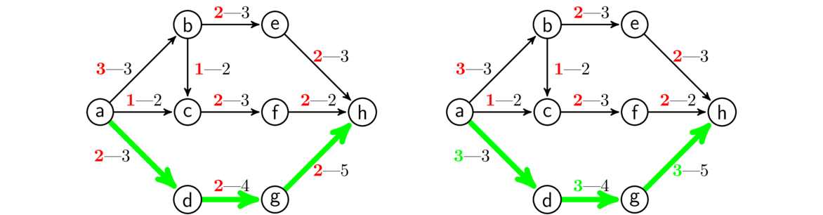
Shown below is an example. The source is a and the sink is h. The first number, highlighted in red on each edge, is the flow value, and the second number is the capacity. The amount of flow on an edge cannot exceed its capacity, and, except for the source and sink, the total amount of flow into a vertex must equal the total amount of flow out of that vertex. That is, the flow passes through the vertices, which neither create nor consume flow. The total amount of flow through the network is called the flow's value. That amount can be found by counting the total flow leaving the source or, equivalently, the total flow entering the sink. Note that the flow below is not optimal, as it would be possible to push more stuff through the network than the current total of 6 units.

Many real problems can be modeled by flow networks. For instance, suppose the source represents a place where we are mining raw materials that we need to get to a factory, which is the sink. The edges represent various routes that we can send the raw materials along, with the capacities being how much material we can ship along those routes. Assuming the transportation network is the limiting factor, we are interested in how much raw material can we get to the factory. Also, many seemingly unrelated problems can be converted into network flow problems. We'll see some examples a little later.

The Max-flow min-cut theorem

Closely related to flows are cuts. A cut is a set of edges whose deletion makes it impossible to get from the source to the sink. We are interested in the sum of the capacities of the edges in cuts. For example, shown below is a cut consisting of edges be, bc, ac, and dg. Its total capacity is 3+2+2+4 = 11.

A famous theorem, called the max-flow min-cut theorem, says that the maximum value of a flow equals the minimum value of a cut. In particular, if we can find a flow and a cut of the same size, then we know that the our flow is a maximum flow (and that the cut is minimum as well).

As an example, in the network below a maximum flow is shown. A total of 8 units of flow move through the network as can be seen by adding up the flow out of the source or the flow into the sink. A minimum cut in this network consists of the edges a → b, a → c, and a → d, whose total capacity is 3+2+3 = 8. Since we have a flow and a cut of the same size, our flow is maximum and our cut is minimum.

The Ford-Fulkerson algorithm

The Ford-Fulkerson algorithm finds max flows and min cuts in a network. We will look at a particular variation of the algorithm called the Edmonds-Karp algorithm.

The basic idea is to start with a flow and use it to find either a better flow or a minimum cut. We do this by looking for paths from the source to the sink along which to improve the flow. The simplest case of such a path is one where all the flow values are below capacity, like in the example below. The flow can be increased by one unit along the path highlighted, as shown on the right.

However, there is another case to consider: backward edges. In the example shown below, we have highlighted a path. Notice that the edge from b to c is backwards. We can steal a unit of flow from that edge and redirect it along the edge from b to e. This gives us a path that increases the flow, as shown on the right.

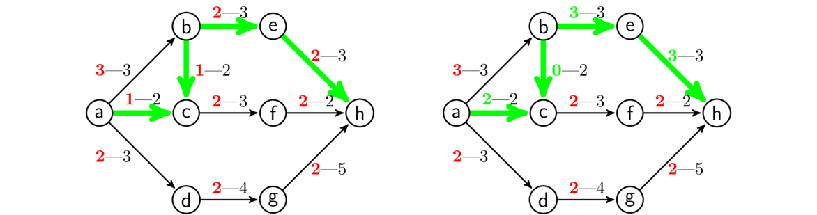
What happens is there are initially 3 units of flow entering vertex b, with 2 units heading to e and 1 unit heading to c. We redirect that 1 unit so that all 3 units go from b to e. This frees up some space at c, which allows us to move a new unit of flow from the source into c, which we can then send into f.

The Ford-Fulkerson algorithm starts with a flow of all zeroes on each edge and continually improves the flow by searching for paths of either of these two types until no such paths can be found. At the same time as it is doing this, it searches for cuts. It does this by maintaining two sets, R and S. The set R is all the “reached” or found vertices and the set S is all the “searched” vertices that we are done with. Initially, R consists of only the source vertex and S is empty.

The algorithm continually searches paths on which to improve the flow as follows: It picks any vertex v of R–S and looks for edges v → u that are under capacity or edges u → v that have positive flow. Whenever it finds such an edge, it adds u to R. Once all the edges involving v are looked at, v is added to S.

If the source is ever added to R, that means we have a path along which we can increase the flow. On the other hand, if it ever happens that R and S are equal, then there are no new vertices left to search from, so we stop and return our flow as a maximum flow, and we return a minimum cut which consists of all the edges with one endpoint in S and one endpoint not in S. Here is the pseudocode for the algorithm:

D = Digraph
B = Backwards Digraph (D with all the edges reversed)
flow = dictionary with edges as keys, all values set to 0
while True:
    R = {source:None}    # R also holds parents
    S = empty set
    while sink is not in R:
        if R==S:         # nothing left to search
            return flow
        pick any vertex v is R that is not in S
        for each neighbor of v:
            if it's a forward edge and under capacity, add it to R
            if it's a backward edge with positive flow, add it to R
        add v to S
    use parents stored in R to trace back the path.
    add 1 to all the forward edges on the path and
    subtract one from all the backward edges

Two notes are in order here:

We have chosen to start with a flow that is initially all 0. This is an easy way to start, but we can start instead with any flow and the algorithm will build on it to find a maximum flow.
We increase the flow by 1 unit at a time. A more sophisticated approach is to increase the flow by as many units as possible along our path. For instance, if we have a path of forward edges, where each flow value is under capacity by at least 5 units, then we could increase the flow on each edge by 5 units.

Coding the algorithm

First, here's a class for a weighted digraph.

class WeightedDigraph(dict):
    def __init__(self):
        self.weight = {}

    def add(self, v):
        self[v] = set()

    def add_edge(self, weight, u, v):
        self[u].add(v)
        self.weight[(u,v)] = weight

Here is the code for the algorithm:

def ford_fulk(V, E, source, sink):
    # set up forwards and backwards digraphs and initialize flow
    flow = {}
    D = WeightedDigraph()
    B = WeightedDigraph()
    for v in V:
        D.add(v)
        B.add(v)
    for w,u,v in E:
        D.add_edge(w,u,v)
        B.add_edge(w,v,u)
        flow[(u,v)] = 0

    while True:
        R = {source:None}
        S = set()
        while sink not in R:
            if R.keys()==S:
                return flow, S
            # pick v in R-S and check for forward edges under cap or backward > 0
            v = next(iter(R.keys()-S))
            for u in D[v]:
                if u not in R and flow[(v,u)] < D.weight[(v,u)]:
                    R[u] = v
            for u in B[v]:
                if u not in R and flow[(u,v)] > 0:
                    R[u] = v
            S.add(v)
        # trace back
        u = sink
        path = [u]
        while R[u] != None:
            if R[u] in D[u]:
                flow[(u,R[u])] -= 1
            else:
                flow[(R[u],u)] += 1
            u = R[u]

A few quick notes about the code:

We store R as a dictionary with keys as vertices and values as those vertices' parents along the path.
We use next(iter(R.keys()-S)) to pick a vertex from R–S. Since R is a dictionary, we need to use R.keys() instead of just R. The next(iter()) part of it is a way to pick an item.
One tricky part of coding this is keeping the order of vertices straight when using the flow variable since sometimes we are looking at forward edges and sometimes we are looking at backward edges.
The last part of the code traces back along the augmenting path we have found. This is similar to path tracking code we have used in other places, like when doing BFS or Dijkstra's algorithm. In fact, the searching that this algorithm does is a variation of BFS.
The running time of the algorithm is O(ve²), where v and e are the number of vertices and edges, respectively.

Here is a little code to test out the algorithm:

V = 'abcdefgh'
E = [(int(w),u,v) for w,u,v in '3ab 2ac 3ad 3be 2bc 3cf 4dg 3eh 2fh 5gh'.split()]
d, S = ford_fulk(V,E,'a','h')
for x in d:
    print(''.join(x), d[x])
print(S)

Examples

For the network we have been looking at throughout this section, let's look at just the final step of the algorithm, where it finds a minimum cut. Shown below is the optimal flow returned by the algorithm.

Once the flow gets to this point, the last step of the algorithm starts with R = {a} and S empty. The algorithm attempts to find paths to increase the flow by searching from a, but it finds none as all the edges from a are at capacity. It then adds a to S and sees that R = S. This stops the algorithm, and the minimum cut consist of all edges from S (which is just a) to vertices not in S, so it consist of edges a → b, a → c, and a → d. Both the flow and the cut have size 8.

Another example

Below is a longer example. The source is a and the sink is g. On the left is our initial flow of all zeroes.

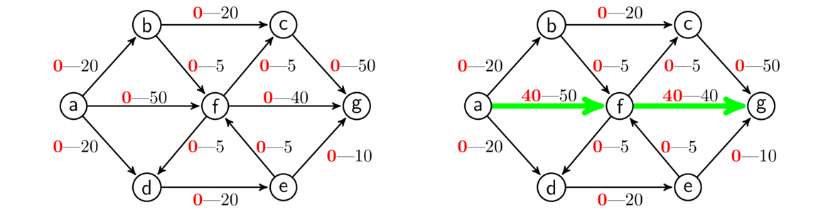
We start with R = {a} and S empty. We search from a and find the edges to b, d, and f under capacity. Thus we add b, f, and d to R, and having finished with a, we add it to S. We then pick anything in R–S, say b, and search from it. From there, we see edges to c and f under capacity, so we add those vertices to R (note that f is already there). Having finished with b, we add it to S, so at this point R is {a, b, f, d, c} and S is {a, b}. We then pick something else in R–S, say f, and search from it. There are some backward edges into f, but as none of those have positive flow, we ignore them. We have forward edges to c, g, and e, so we add them to R.

At this point, the sink, g, has been added to R, which means we have a path along which we can increase the flow, namely afg. Our algorithm keeps track of the fact that we reached f from a and that we reached g from f, and uses that to reconstruct the path. Then we can increase the flow by 1 along edges af and fg, or if we want to be more efficient, we an actually increase it by 40 units on both edges, as shown above on the right.

We then reset R to {a} and S to being empty and repeat the search. Several more searching steps follow until we arrive at the maximum flow shown below on the left.

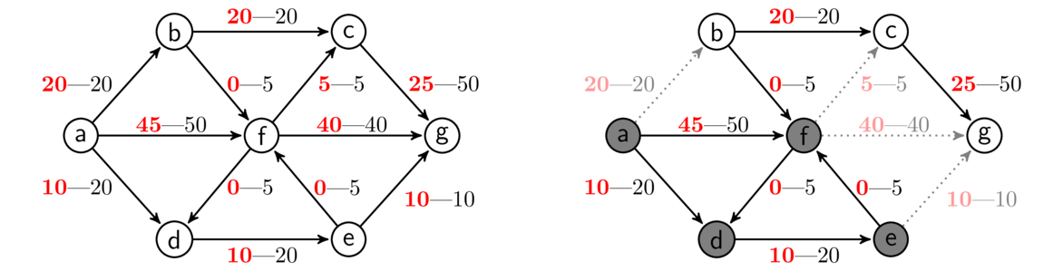
At the last step, we start again with R = {a} and S empty. The edges from a to f and d are below capacity, so we add them to R, and then we add a to S. Next, we pick something in R–S, say f. All of the new backward edges into f have 0 flow, and the only forward edge below capacity is to d, so we don't add anything new to R. So now R = {a, f, d}, S = {a, f}, and we explore from d. This adds only e to R. Exploring from e adds nothing new to R, and we end up with R and S both equal to {a, f, d, e}.

Since R = S, the algorithm ends, and our minimum cut consists of all the edges directed from vertices in S to vertices not in S, specifically edges ab, fc, fg, and eg, for a total capacity of 20+5+40+10 = 75, the same as the value of the flow. The minimum cut is shown above on the right.

Applications

The Max-flow min-cut theorem can be used for a variety of purposes. One can imagine various practical applications for shipping things from one location to another. There are also applications within graph theory as many problems can be transformed into network flow problems.

For instance, we can use network flow to find maximum matchings. Suppose we have four people a, b, c, and d, and four jobs A, B, C, and D. Each person can do certain jobs but not others. We want to know if there is a way to match people to jobs so that everybody gets a job they can do. We can create a bipartite graph, where one part of the graph is for people, the other is for jobs, and we have an edge from each person to each job they can do. We want to find four edges that each go from a different person to a different job.

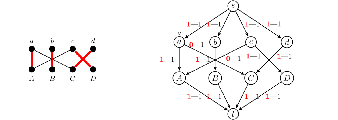
On the left above is an example matching. On the right above, we show how to turn this into a network flow problem. Direct all edges so they point from people to jobs. Add a source vertex s with edges directed from s to every person. Add a sink vertex t with edges directed from every job into t. Give every edge a capacity of 1. We then find a maximum flow in this network. A maximum matching is given by taking all the edges in the middle that have a flow value of 1. The total value of the flow equals the size of the matching.

It turns out that this same approach can be used to solve the vertex covering problem on bipartite graphs. This is where we want to know the least amount of vertices such that every edge has at least one of those vertices as an endpoint. The vertices (excluding the source and sink) that belong to the minimum cut end up forming a minimum vertex cover.

Another nice example of network flow is to find the number of distinct paths in a graph from one vertex to another. For instance, in the graph below, if we want the number of paths from s to t, we could turn the graph into a network by making s the source, making t the sink, and adding capacity 1 to all the edges.

The maximum number of disjoint paths would then be equal to the total value of the flow reaching t. The minimum cut would answer another interesting problem. It would tell us the minimum number of edges we need to remove in order to disconnect s from t. That tells us how well connected our network is. For this example, we get a minimum cut of size 3, which tells us that we can remove any 2 edges from the graph and it will still be possible to get from s to t. Both the number of disjoint paths and the number of edges needed to disconnect s from t have important applications to reliability of computer networks and other kinds of networks.

There are many more applications of network flow, even to seemingly unrelated problems like determining when a sports team is eliminated from winning their division. For algorithms in general, an important technique is this idea of turning a problem into another one that we know how to solve (sometimes called a reduction).

Flows with multiple sources and sinks

It is not too hard to handle multiple sources and sinks. We create a single “super source” with edges directed towards every source and add infinite (or extremely high) capacity to each edge. A similar “super sink” can be added with edges of infinite capacity directed from every sink to the super sink.