Shortest Paths
We'll look at several algorithms for finding the shortest (least cost) path between two vertices in a weighted graph. Shortest paths have a lot of applications, the most well known of which is probably GPS navigation.
Floyd-Warshall algorithm
The Floyd-Warshall algorithm works on the adjacency matrix representation of a graph. The rows and columns in the adjacency matrix are the vertices. For an ordinary graph, the adjacency matrix stores a 1 to indicate vertices are adjacent and a 0 to indicate they aren't. For a weighted graph with the weights representing distances, this changes a bit. An entry in the row for vertex u and the column for vertex v will be the weight of edge uv if it exists. If there is no edge, then the entry is ∞ to indicate it is not possible to get directly from u to v. The entries along the main diagonal are all set to 0 since the distance from a vertex to itself is 0. An example is shown below.

Here is code that creates a weighted adjacency matrix. The parameters are a set of vertices V and a set of edges E, organized as tuples of the form (weight, u, v). We use float('inf') to get a Python representation of infinity. In Java, you could use Integer.MAX_VALUE or Double.MAX_VALUE.
def create_adjacency_matrix(V, E):
    M = [[float('inf')]*len(V) for v in V]
    for i in range(len(V)):
        M[i][i] = 0
    for weight, u, v in E:
        M[V.index(u)][V.index(v)] = weight
        M[V.index(v)][V.index(u)] = weight
    return M
Here is a some code that prints out an adjacency matrix.
def pr(M):
    for i in range(len(M)):
        for j in range(len(M[0])):
            print(M[i][j], end=' ')
        print()
The main idea of the Floyd-Warshall algorithm is that it loops over all the vertices k in the graph and for each one, it loops over all pairs of vertices i and j and sees if it can improve the current best distance/path from i to j by instead going through k. Specifically we see if we can improve the path from i to j by taking the current best path from i to k and then taking the current best path from k to j. Here is code for it. This simple version only finds the distances and not the actual paths.
def floyd_warshall(M):
    C = copy.deepcopy(M) # make a copy since we will be modifying the matrix
    for k in range(len(C)):
        for i in range(len(C)):
            for j in range(len(C)):
                if C[i][k] + C[k][j] < C[i][j]:
                    C[i][j] = C[i][k] + C[k][j]
    return C
Let's look at an example. We will use the graph below. Its adjacency matrix is shown on the right.

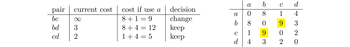
The outer loop of the algorithm has the variable k run through each of the vertices in the graph. The two inner loops run over all pairs of vertices, seeing if we can use k to improve the path between each pair. We start with k = 0, corresponding to trying to improve paths by using vertex a. We look at all pairs of vertices in the graph not involving a.
For the pair bc, there is currently no path from b to c, so its current cost is ∞. We look at going through a, specifically b to a to c. The ba cost is 8 and the ac cost is 1, so the total cost here is 9, which is an improvement over ∞. In the code, this corresponds to the k = 0, i = 1, j = 2 step. The other two pairs bd, and cd will see no improvement from using a. This is summarized in the table below on the left and the change to the matrix is highlighted on the right.
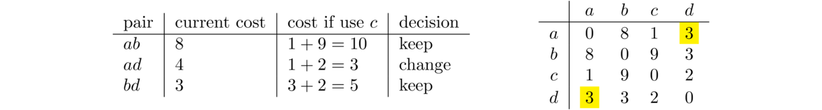
The next step through the outer loop, with k = 1, is about using vertex b to improve paths. It turns out that nothing improves here, so we move on to k = 2, looking at vertex c. There is one path that improves. The current cost from a to d is 4, and we can improve that by going from a to c to d for a cost of 3. To do this, be sure to use the new version of the matrix and not the graph. The matrix keeps track of the current best paths, and we want to know about total path costs, not edge costs. Here is the summary of the k = 2 step.
The last step uses d to improve paths. There are two that improve. The path from a to b can be improved by using the path from a to d and the path from d to b. Note that this isn't the direct path a → d → b. Instead it runs a → c → d → b. The path from a to d had already been improved when examining vertex c. In general, the matrix is continually improved, step by step. We also can improve the path from b to c by using d.
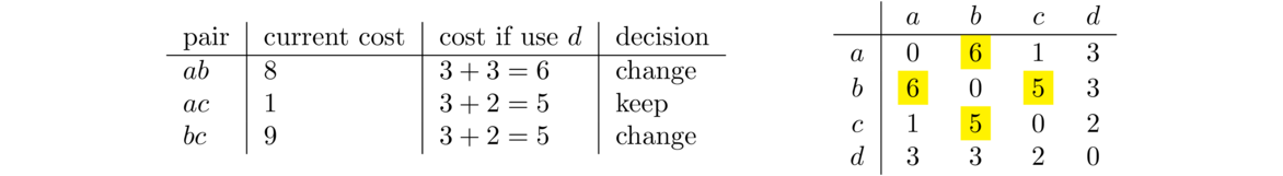
The final matrix shown at the right above is our desired result. It tells us the shortest distances from each vertex to each other vertex. Though we won't do so, it's not too much work to modify the code to also keep track of the shortest paths themselves instead of only the distances.
Bellman-Ford algorithm
This is an algorithm for finding the distances/shortest paths from a single starting vertex to all other vertices in a graph. A version of it is used in the Routing Internet Protocol (known as RIP), used by routers in smaller networks to build their routing tables. The algorithm starts by creating a dictionary d that will hold the distances from the start to everything else. Initially, the distance from the start to itself is 0 and all the other distances are ∞. We then run the following code:
for i in range(len(G)-1):
    for u in G:
        for v in G[u]:
            w = G.weight[(u,v)]
            if d[u] + w < d[v]:
                d[v] = d[u] + w
The for u in G loop goes over all the vertices in the graph. For each of those vertices, the innermost loop looks at all the edges going out from it. If taking that edge (call it uv) improves the current distance from the start to v, then we update the dictionary entry for v. The code does that by comparing d[u] + w to d[v] and replacing d[v] with d[u] + w if the latter is smaller.
Once we go all the way through the vertices, the dictionary should be in a lot better shape than where it started, but it might not be all the way done. So we run the two inner loops again. In fact, to guarantee we get all the least distances, we have to run things len(G)–1 times, although often things will be done after just one or two iterations. Below is an example of the process. We'll use this graph with a as the starting vertex.

The table below shows how the dictionary evolves during the i = 0 iteration of the outer loop. The u = a, u = b entries indicate the state of the dictionary after each iteration of the second loop. Changes are highlighted.
| a | b | c | d | e | f | g | |
| init | 0 | ∞ | ∞ | ∞ | ∞ | ∞ | ∞ |
| u = a | 0 | \h{12} | \h{1} | \h{4} | ∞ | ∞ | ∞ |
| u = b | 0 | 12 | 1 | 4 | \h{19} | \h{14} | ∞ |
| u = c | 0 | 12 | 1 | \h{3} | \h{4} | 14 | ∞ |
| u = d | 0 | 12 | 1 | 3 | 4 | 14 | ∞ |
| u = e | 0 | \h{11} | 1 | 3 | 4 | 14 | \h{6} |
| u = f | 0 | 11 | 1 | 3 | 4 | 14 | 6 |
| u = g | 0 | 11 | 1 | 3 | 4 | \h{7} | 6 |
| a | b | c | d | e | f | g | |
| … | |||||||
| u = f | 0 | \h{9} | 1 | 3 | 4 | 7 | 6 |
| … |
def bellman_ford(G, start):
    parent = {start: None}
    d = {v: float('inf') for v in G}
    d[start] = 0

    for i in range(len(G)-1):
        for u in G:
            for v in G[u]:
                weight = G.weight[(u,v)]
                if d[u] + weight < d[v]:
                    d[v] = d[u] + weight
                    parent[v] = u
    return d, {v:path(parent, v) for v in G}

def path(parent, v):
    P = [v]
    while parent[v] != None:
        v = parent[v]
        P.append(v)
    P.reverse()
    return P
Dijkstra's algorithm
In this section we will look at what is probably the most well-known shortest path algorithm—Dijkstra's algorithm. To see how it works, consider the example below in which we are looking for the shortest path from vertex a to vertex g.
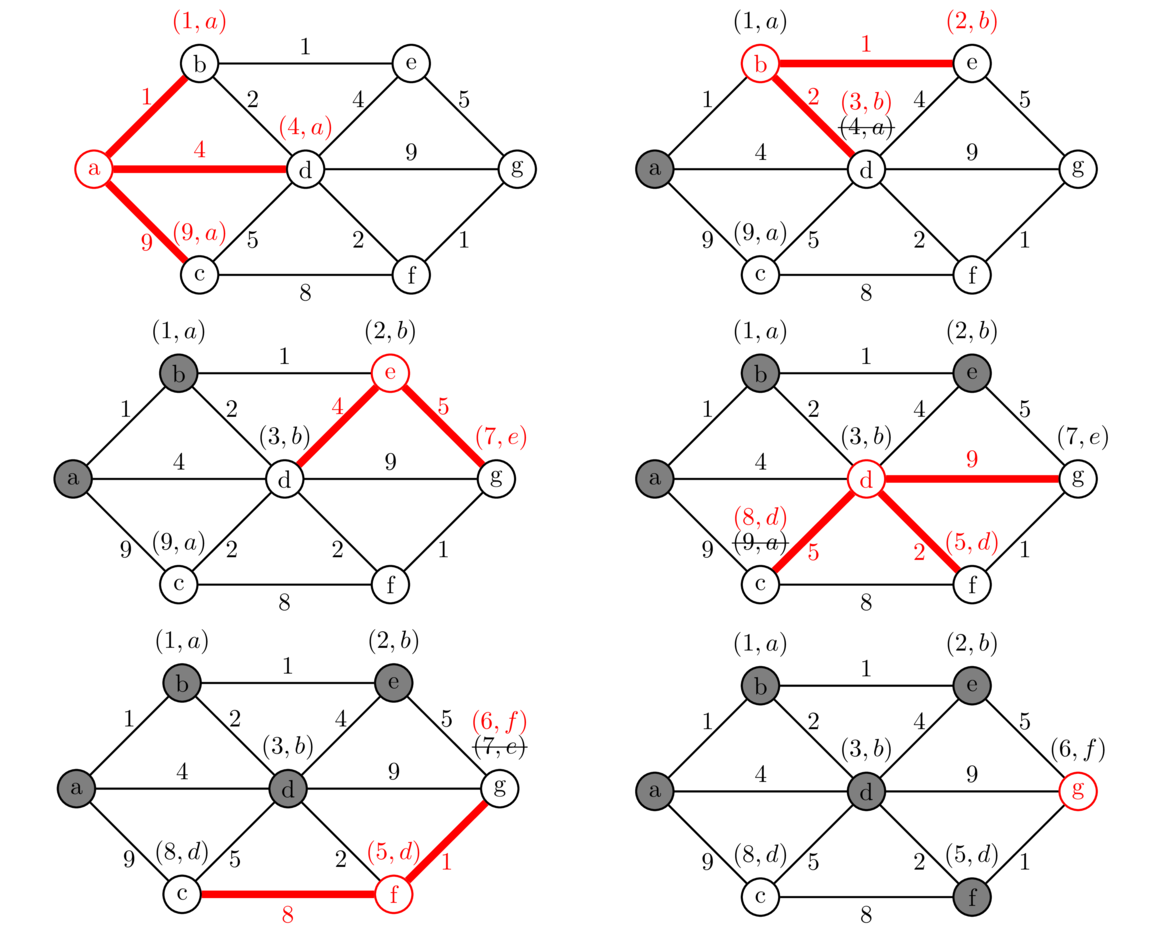
We start from vertex a, visiting each of its neighbors and labeling them with the cost from a, along with an a to indicate that we found them via vertex a. We then mark a as “searched” meaning we will not visit it any more.
We next pick the neighbor of a that was labeled with the smallest cost and visit its neighbors. This is vertex b. Currently, we know that we can get to b from a with a total cost of 1. Since it costs 1 to get from b to e, we label e as (2, b) indicating that we can get from a to e for a total cost of 2 with b indicating that we got to e via vertex b. Similarly, we can get to vertex d with a total cost of 3 by going through b. That vertex d has already been labeled, but our route through b is cheaper, so we will replace the label on d with (3, b). If the cost to d through b had been more expensive, we would not change the label on d. Also, we ignore the edge from b back to a since a has been marked as “searched”. And now that we're done with b, we mark it as “searched”.
We continue this process for the other vertices in the graph. We always choose the next vertex to visit by looking at all the vertices in the graph that have been labeled but not marked as visited, and choose the one that has been labeled with the cheapest total cost, breaking ties arbitrarily. The next vertex to visit would be e, as its total cost is currently 2, cheaper than any other labeled vertex. After a few more steps we get to the point that g is the cheapest labeled vertex. This is our stopping point. Once our goal vertex has the cheapest label, no other route to that goal could possibly be better than what we have. So we stop there, even though we haven't necessarily explored all possible routes to the goal.
We then use the labels to trace the path backward to the start. For instance, at the end g was labeled with (6, f), so we trace backward from g to f. That vertex f was labeled with (5, d), so we trace backward to d and from there back to b and then a, giving us the path abdfg with a total length of 6 as the shortest path.
Algorithm description
Here is a short description of the algorithm in general. Assume the start vertex is called a. The algorithm labels a vertex v with two things: a cost and a vertex. The cost is the current shortest known distance from a, and the vertex is the neighbor of v on the path from a to v that gives that shortest known distance. The algorithm continually improves the cost as it finds better paths to v. Here are the steps of the algorithm.
- Start by setting the cost label of each neighbor of a to the cost of the edge from a to it, and set its vertex label to a. Mark a as “searched.” We will not visit it again.
- Then pick the labelled vertex v that has the smallest cost, breaking ties however we want. Look at each neighbor of v. If the neighbor is unlabeled, then we label it with a cost of c plus the weight of the edge to it from v. Its vertex label becomes v. If the neighbor is already labeled, we compare its current cost label with c plus the weight of the edge to it the neighbor from v. If this is no better than the neighbor's current cost label, then we do nothing more with this vertex. Otherwise, we update the label's cost with this new cost and update the neighbor's vertex label to v. We repeat this for every unsearched neighbor of v and then label v itself as “searched,” meaning we will not visit it again.
- The algorithm continues this way, at each step picking the unsearched labelled vertex that has the smallest cost and updating its neighbors' labels as in Step 2.
- The algorithm ends when the labelled vertex with the smallest cost is the destination vertex. That cost is the total cost of the shortest path. We then use the vertex labels to trace back to find the path from the start to the destination. The destination vertex's vertex label is the second-to-last vertex on the path. That vertex's vertex label is the third-to-last vertex on the path, etc.
Below is code implementing Dijkstra's algorithm. It uses heap functions from the heapq library.
def dijkstra(G, start, goal):
    info = {start: {'cost':0, 'parent':None}}
    heap = [(0, start)]

    while len(heap) > 0:
        _, w = heappop(heap)

        if w == goal:
            P = [w]
            while info[w]['parent'] != None:
                w = info[w]['parent']
                P.append(w)
            P.reverse()
            return P, info[goal]['cost']

        for n in G[w]:
            weight = G.weight[(w,n)]
            if n not in info or info[w]['cost'] + weight < info[n]['cost']:
                info[n] = {'cost':info[w]['cost'] + weight, 'parent':w}
                heappush(heap, (info[w]['cost'] + weight, n))
    return []
The info dictionary corresponds to the labels on the vertices from the algorithm description above. We use a heap to allow us to efficiently choose the vertex with the smallest cost. In order to do this, we store the items in the heap as tuples with the first value being the cost and the second being the vertex. This allows the heap to store things based on the cost. When we pop the item off the heap, we don't care anymore about the cost, so we use the _ special variable to indicate to people reading the code that we are ignoring it.
Recall that the algorithm ends when the vertex with the cheapest cost is the goal. That's what the first if statement is for. The code in that if block uses the info dictionary to trace back the path to the start. The main part of the algorithm comes at the bottom of the loop. For each neighbor of the vertex popped off the heap, we check to see if it hasn't been found yet or if we can improve the current cost to it. If either of these is true, then we update the info dictionary with the new cost and push the vertex onto the heap. It might happen that the same vertex is pushed onto the heap multiple times with different costs, but that won't be an issue. If it happens that the same vertex is popped multiple times from the heap, any time after the first it will just be a little wasted time. To speed things up a little, a check could be added to the code right after the pop statement.
An application to board searching
In some situations, explicitly creating a graph might be more work than is needed. It might even turn out that the graph is too big to fit in memory. Instead, we can write a function that returns the neighbors of a vertex. The version of Dijkstra's algorithm below has been rewritten slightly to use this approach. In place of the graph parameter, we have a get_neighbors function that returns the neighbors of a given vertex. We'll have it return the neighbors in a tuple of the form (weight, neighbor), with the weight being the weight of the hypothetical edge leading to the neighbor. To get Dijkstra's algorithm to work with this function, we only need to change the loop over the neighbors in a few small places. See below.
def dijkstra(get_neighbors, start, goal):
    info = {start: {'cost':0, 'parent':None}}
    heap = [(0, start)]

    while len(heap) != 0:
        _, w = heappop(heap)
        if w == goal:
            P = []
            while w != None:
                P.append(w)
                w = info[w]['parent']
            P.reverse()
            return P, info[goal]['cost']

        for weight,n in get_neighbors(w):
            if n not in info or info[w]['cost'] + weight < info[n]['cost']:
                info[n] = {'cost':info[w]['cost'] + weight,
                           'parent':w}
                heappush(heap, (info[n]['cost'], n))

    return []
Let's use this version of Dijkstra's algorithm to find shortest paths on a square grid, like a checkerboard. We can think of the cells of the boards in terms of their coordinates in a (row, column) format with (0, 0) in the upper left, (0, 1) directly to the right of it, (1, 0), directly below, etc.
Here is some code to create a board. To make it quick to change the board around, we put it into a string, and the line of code at the bottom explodes it into a 2-dimensional array. The - characters will be open cells and the * characters will be walls.
textboard = """
------*-------------
------*-------------
------*-------------
------*-------------
------*-------------
------*-------------
------*-------------
------*-------------
-------------*------
-------------*------
-------------*------
-------------*------
-------------*------
-------------*------
-------------*------
-------------*------
-------------*------
-------------*------
-------------*------
-------------*------"""
board = [list(x) for x in textboard[1:].split('\n')]
Here is a function that returns all the neighbors of a cell in the horizontal, vertical, and diagonal directions. There are eight possible neighbors, though some of them will lie off the end of the board. The last line filters those out. It assumes the board is size 20, but that can be easily changed if needed. The code also uses the filter to only return neighbors that are open cells, not walls.
def get_neighbors_hvd(v):
    r, c = v
    N = [(r-1,c-1),(r-1,c),(r-1,c+1),
         (r,c-1),(r,c+1),
         (r+1,c-1),(r+1,c),(r+1,c+1)]
    return [(1,(r,c)) for r,c in N if 0<=r<20 and 0<=c<20 and board[r][c] != '*']
Finally, we can call Dijkstra's algorithm and display the path it finds. It will avoid walls and return the shortest path from the upper left to the lower right.
P = dijkstra(get_neighbors_hvd, (0,0), (19,19))[0]
for i in range(len(P)):
    r,c = P[i]
    board[r][c] = str(i + 1)

# display the board
for r in range(len(board)):
    for c in range(len(board[r])):
        print('{:>2s}'.format(board[r][c]), end=' ')
    print()
A* search
There is a very small change that we can make to Dijkstra's algorithm that can give a vast improvement. Recall that Dijkstra's algorithm always chooses the vertex with the cheapest current cost from the start as the next one to explore. But it doesn't account for the goal in any way. A* search uses a function, called a heuristic, to estimate the distance to the goal. It uses that information along with the current cost from the start in deciding which vertex to visit next. Here is code implementing this, based on the get_neighbors version of Dijkstra's algorithm:
def astar(get_neighbors, start, goal, heuristic):
    info = {start: {'cost':0, 'parent':None}}
    heap = [(0, start)]

    while len(heap) != 0:
        _, w = heappop(heap)
        count += 1
        if w == goal:
            P = []
            while w != None:
                P.append(w)
                w = info[w]['parent']
            P.reverse()
            print('A* examined', count)
            return P, info[goal]['cost']

        for weight,n in get_neighbors(w):
            if n not in info or info[w]['cost'] + weight < info[n]['cost']:
                info[n] = {'cost':info[w]['cost'] + weight,
                           'parent':w}
                heappush(heap, (info[n]['cost'] + heuristic(n,goal), n))

    return []
The only change from the Dijkstra's code is that the function now takes a heuristic as a parameter, and it uses it in the heappush call. Instead of just using the cost, we use the cost plus the heuristic. The result is that A* will typically find the shortest path considerably faster than Dijkstra's algorithm. We can use A* with the board-searching code above to see how it does. We need a heuristic function. A simple one that works is the Manhattan distance. Imagine walking from a cell to the goal along the grid, going horizontally and or vertically (like walking along the gridded streets of Manhattan). The Manhattan distance is the total distance traveled this way, the sum of the total horizontal and vertical distance traveled. Here is code for it:
def manhattan(v, goal):
    r, c = v
    rg, cg = goal
    return abs(rg-r) + abs(cg-c)
The hard part of the A* algorithm usually involves coming up with a good heuristic function. The A* algorithm will return the shortest path as long as the heuristic used is guaranteed to never overestimate the distance to the goal. People use the term admissible to describe a heuristic that doesn't overestimate. If a non-admissible heuristic is used, A* will still find a path, but there's no guarantee that it will be optimal.
If you add a count variable to the functions to count every time a vertex is popped off the heap, you'll see that for the example board above, Dijkstra's has to examine 380 out of the 400 vertices before it finds the shortest path. A* needs to examine only 111.
info dictionary can be replaced by a dictionary that just keeps track of parents along the paths it finds.
def greedy_best(get_neighbors, start, goal, heuristic):
    parent = {start:None}
    heap = [(0, start)]
    count = 0

    while len(heap) != 0:
        _, w = heappop(heap)
        count += 1
        if w == goal:
            P = []
            while w != None:
                P.append(w)
                w = parent[w]
            P.reverse()
            return P

        for weight,n in get_neighbors(w):
            if n not in parent:
                parent[n] = w
                heappush(heap, (heuristic(n,goal), n))

    return []
On the board example used above, A* examines 111 vertices and greedy best first search examines 92. However, it doesn't find the shortest path. It finds a path of length 32, while the shortest is of length 28. In general, greedy best first search will run more quickly than the other two algorithms, and it often won't find the shortest path.
A nice exercise is to try to use these algorithms to solve the 8 puzzle. This is a puzzle where tiles numbered 1 to 8 are arranged on a 3 × 3 board in a random order. The other spot on the board is empty, and tiles can be slid around using that empty spot. The goal is to rearrange the tiles into numerical order. In some code I wrote, A* ended up averaging about a 10 times speedup over Dijkstra and greedy best first search about a 10 times speedup over A*, though greedy best first search tends to return paths that are in some cases several times as long as the shortest path.
Comparing the shortest path algorithms
Let's compare the Floyd-Warshall, Bellman-Ford, and Dijkstra's algorithms. We'll look at running times in terms of v and e, the number of vertices and edges, respectively, in the graph. In the worst case scenario, where every vertex is adjacent to every other vertex, e = v(v–1)/2. In a better scenario, maybe each vertex is adjacent an average of 10 other vertices. In that case, e is approximately 5v.
The Floyd-Warshall algorithm runs in O(v3) time, and finds the shortest paths from every vertex to every other vertex. It is the slowest of the three algorithms, but it also accomplishes the most of all of them.
The Bellman-Ford algorithm finds shortest paths from a vertex to all other vertices. Its running time is O(ve). So this is O(v3) in the worst case and O(v2) in a more ordinary case. One benefit of Bellman-Ford over Dijkstra is that Bellman-Ford can handle graphs with negative edge weights, unlike Dijkstra.
Dijkstra's algorithm finds the shortest path from one vertex to a specific goal vertex, but if we run the code without a goal vertex and let the while loop go until the heap empties out, then Dijkstra's will find shortest paths from the start vertex to every other vertex, just like the Bellman-Ford algorithm. Dijkstra's algorithm has running time O((v+e) log v). So this is O(v2 log v) in the worst case and O(v log v) in a not-so-bad case. This can be improved a bit by using a fancier version of a heap called a Fibonacci heap.
Probably the most obvious real-world use of these algorithms would be for GPS navigation. An additional optimization called contraction hierarchies is used for GPS navigation. The basic idea of this is on a road network there are many roads that will not be useful in finding the shortest path. For instance, along a main road, there are often side roads that go into housing developments that don't improve shortest paths. Some preprocessing can be done to the graph to replace sections of the graph like this with shortcut edges. This cuts down on the number of vertices that need to be searched, improving the running time.
Appendix
Below is code for the WeightedGraph class covered in the notes on spanning trees. It is needed for the Bellman-Ford and Dijkstra code.
class WeightedGraph(dict):
    def __init__(self):
        self.weight = {}

    def add(self, v):
        self[v] = set()

    def add_edge(self, weight, u, v):
        self[u].add(v)
        self[v].add(u)
        self.weight[(u,v)] = self.weight[(v,u)] = weight