Sorting
Sorting is worth studying for a few reasons: (1) it's one of the fundamental parts of computer science that computer scientists are expected to be familiar with, (2) ideas used in some of the algorithms are useful elsewhere, and (3) there are some sorting algorithms that can, in some special cases, outperform the sorting methods built into programming languages. We'll start by looking at how to use some of the more advanced features of those built-in sorting methods.
Sorting in Python
If you have a list L in Python, you can use L.sort() to sort it. Another option is to use sorted(L). The difference is that the former will change L, while the latter will return a new sorted copy of L. To sort a list in reverse order, use L.sort(reverse=True). This and other keyword arguments also work with the sorted function.
key keyword argument is used for that. For instance, to sort a list of strings by length, so that they are organized from shortest to longest, use L.sort(key=len). The argument to the key function will be a function that tells how the sorting is to be done. If we want to sort a list of strings by how many of the letter z they contain, we could do the following:
def num_z(s):
    return s.count('z')

L = ['zoo', 'buzz', 'pizazz', 'pizza', 'cat', 'zzzzz!', 'computer']
print(sorted(L, key=num_z))
There is a one-line shortcut for the above:
print(sorted(L, key=lambda s:s.count('z')))
This uses the lambda keyword, which is a way to create an anonymous function. The idea is that the z-counting function is not something we need anywhere except as a sorting key, so there is no need to go through the trouble of creating a full function. Instead, Python's lambda keyword allows us to create an unnamed function and put it directly into the call to the sorting function.
I personally use sorting by a key most often for sorting tuples. Suppose we have a list of tuples like [(4,5), (2,3), (1,9), (2,6), (7,1), (8,2)]. Sorting this list without a key will sort it by the first item in each tuple, with ties being broken by moving to the second item and further if necessary for larger tuples.
Sometimes, it is helpful to sort by a different entry. To sort a list L by the second entry (index 1 of the tuple), we can use the line below. The sorting key is the value of the item at index 1 of the tuple.
L.sort(key=lambda t:t[1])
Here how to sort the keys of a dictionary by their corresponding values:
sorted(d, key=d.get)
You can also use key=lambda x:d[x] for the key function above. Finally, we can sort a list of objects according to one of the fields in the objects. For instance, if the objects all have a field called age, then the following will sort based on that:
L.sort(key = lambda x:x.age)
Sorting in Java
There is an array sorting method in java.util.Arrays. Here is an example of it:
int[] a = {3,9,4,1,3,2};
Arrays.sort(a);
When working with lists, one approach is Collections.sort. Here is an example:
List<Integer> list = new ArrayList<Integer>();
Collections.addAll(list, 3,9,4,1,3,2);
Collections.sort(list);
In Java 8 and later, lists have a sorting method, as shown below:
List<Integer> list = new ArrayList<Integer>();
Collections.addAll(list, 3,9,4,1,3,2);
list.sort();
Collections.sort(list, new Comparator<String>() {
    public int compare(String s, String t) {
        return s.length() - t.length(); }});
This uses something called a Comparator. The key part of it is a function that tells how to do the comparison. That function works like the compareTo method of the Comparable interface in that it returns a negative, 0, or positive depending on whether the first argument is less than, equal to, or greater than the second argument. The example above uses an anonymous class. It is possible, but usually unnecessary, to create a separate, standalone Comparator class. Things are much easier in Java 8. Here is code to sort a list of strings by length:
list.sort((s,t) -> s.length() - t.length());
In place of an entire anonymous Comparator class, Java 8 allows you to specify an anonymous function. It basically cuts through all the syntax to get to just the part of the Comparator's compare function that shows how to do the comparison.
Say we have a class called Record that has a field called age, and we want to sort a list of records by age. We could use the following:
Collections.sort(list, new Comparator<Record>() {
    public int compare(Record r1, Record r2) {
        return r1.age - r2.age; }});
In Java 8 and later, we can do the following:
list.sort((r1, r2) -> r1.age - r2.age);
If we have a getter written for the age, we could also do the following:
list.sort(Comparator.comparing(Record::getAge));
Suppose we want to sort by a more complicated criterion, like by last name and then by first name. The following is one way to do things:
Collections.sort(list, new Comparator<Record>() {
            public int compare(Record r1, Record r2) {
                if (!r1.lastName.equals(r2.lastName))
                    return r1.lastName.compareTo(r2.lastName);
                else
                    return r1.firstName.compareTo(r2.firstName); }});
In Java 8 and later, we can use the following:
list.sort(Comparator.comparing(Record::getLastName).thenComparing(Record::getFirstName));
Uses for sorting
Here is a list of some places sorting can be helpful:
- Once a list is sorted, certain algorithms become faster. For instance, we can use a fast binary search instead of a slow linear search once the list is sorted. This speed gain needs to be balanced with the fact that sorting the list takes time. However, if you're planning to do many searches, then it makes sense to sort the list once at the start.
- Finding the largest and smallest things in a sorted list is easy, as is finding the second-largest, the median (middle value), and many other things.
- A common task is to determine if a list has repeats. If the list is already sorted, a quick way to do that is to loop over the list and see if any pair of elements next to each other are equal. This runs in O(n) time. An alternate approach is to convert the list to a set and see if the list and set have the same length. This is can be done by checking if
len(L) == len(set(L))in Python. This is slower than the loop approach described above, but it is quicker to code. - Finding the two closest things together in a list can be done similarly to the above. Once the list is sorted, the two closest things together will be next to each other in the list.
Insertion sort
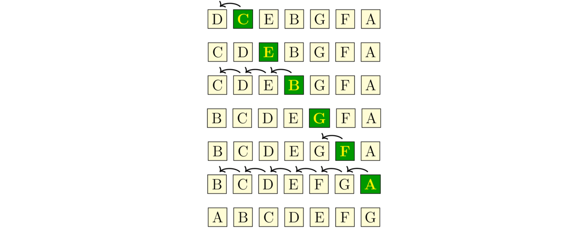
Insertion sort is an O(n2) algorithm that is possibly the fastest common sorting algorithm for small lists of up to maybe a few dozen elements. For large lists, other algorithms are much faster. Insertion sort is also a very good sort for lists that are already almost in sorted order.To understand the basic idea, suppose we have a stack of papers we want to put into in alphabetical order. We could start by putting the first two papers in order. Then we could put the third paper where it fits in order with the other two. Then we could put the fourth paper where it fits in order with the first three. If we keep doing this, we have what is essentially insertion sort.
To do insertion sort on an array, we loop over the indices of the array running from 1 to the end of the array. For each index, we take the element at that index and loop back through the array towards the front, looking for where the element belongs among the earlier elements. These elements are in sorted order (having been placed in order by the previous steps), so to find the location we run the loop until we find an element that is smaller than the one we or looking at or fall off the front of the array. The figure below shows it in action.
Below is code for insertion sort in Python. This code will sort the caller's list instead of making a separate copy and sorting that. It's not hard to modify the code to make a copy if that's what you want.
def insertion_sort(L):
    for i in range(1, len(L)):
        current_val = L[i]
        j = i
        while j > 0 and current_val < L[j-1]:
            L[j] = L[j-1]
            j -= 1
        L[j] = current_val
We see the nested loops in the code above, showing that insertion sort is O(n2) in the worst case. That worst case would be a list in reverse sorted order. Insertion sort turns out to be O(n2) in the average case as well. The best case for insertion sort is if the list is already sorted. In that case, the inner loop never runs, and it's O(n). If the list is mostly sorted except for a few elements a little out of place, we are close to this best case, and the running time is still pretty good.
Mergesort
Mergesort is a widely used sort that runs in O(n log n) time for all inputs. A variation of it called Timsort is the sorting algorithm used by Python and by some Java library functions.
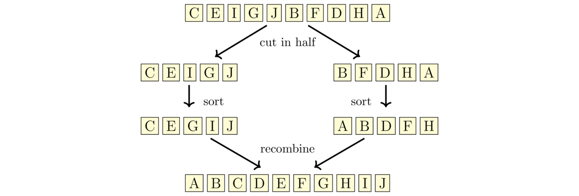
Mergesort works as follows: We break the array into two halves, sort them, and then merge them together. The halves themselves are sorted with mergesort, making this is a recursive algorithm. For instance, say we want to sort the string CEIGJBFDHA. We break it up into two halves, CEIGJ and BFDHA. We then sort those halves (using mergesort) to get CEGIJ and ABDFH and merge the sorted halves back together to get ABCDEFGHIJ. See the figure below:
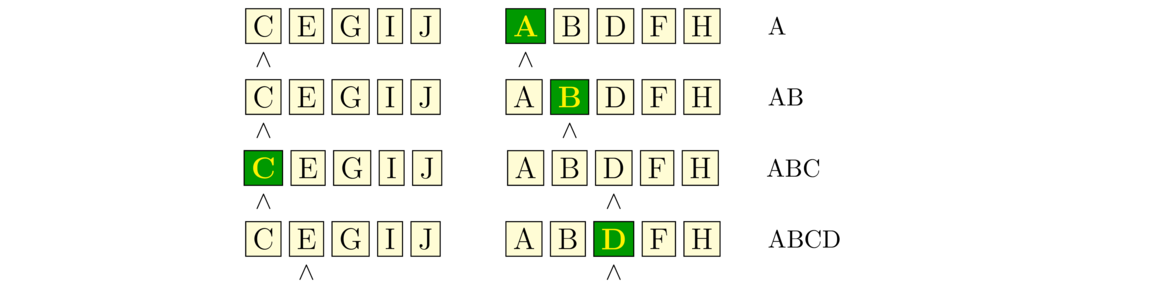
The way the merging process works is we have position markers (counters) for each of the two halves, each initially at the starts of their corresponding halves. We compare the values at the markers, choose the smaller of the two, and advance the corresponding marker. We repeat the process until we reach the end of one of the halves. After that, we append any remaining items from the other half to the end. The first few steps are shown below:
Below is one way to code mergesort in Python. It uses the merge function built into Python in the heapq library.
def mergesort(L):
    if len(L) <= 1:
        return

    left = L[:len(L)//2]
    right = L[len(L)//2:]

    mergesort(left)
    mergesort(right)

    for i,x in enumerate(merge(left, right)):
        L[i] = x
Mergesort is naturally coded recursively. The base case to stop the recursion is lists of length 0 or 1, which don't need to be sorted. We then break the list into its left and right halves, mergesort those, and then merge the result back together. The enumerate function is just a way to have a loop that gets both the index and the item at once from looping over the object returned by the merge function. If we really want to see how mergesort works, without relying on Python's merge function, below is a different approach.
def mergesort(L):
    mergesort_helper(L, [None]*len(L), 0, len(L))

def mergesort_helper(L, M, left, right):
    # Base case to end the recursion
    if right-left <= 1:
        return

    # Recursive breakdown
    mid = (left + right) // 2
    mergesort_helper(L, M, left, mid)
    mergesort_helper(L, M, mid, right)

    # Make a copy of L into M
    for i in range(left, right):
        M[i] = L[i]

    # Merging code
    x, y, z = left, mid, left
    while x < mid and y < right:
        if M[x] < M[y]:
            L[z] = M[x]
            x += 1
        else:
            L[z] = M[y]
            y += 1
        z += 1

    while x < mid:
        L[z] = M[x]
        x += 1
        z += 1

    while y < right:
        L[z] = M[y]
        y += 1
        z += 1
The merging process could be coded in a simpler way, but it would end up being slow due to a bunch of new lists being continually created to help with the moving. The code above creates a single separate array M and uses that as a sort of workspace for moving things around in the merging process. Because of this, we end up needing to add M and two other variables as parameters to the recursive method. These extra parameters change how the user would call the function, so we use a helper function.
The basic idea behind why the running time is O(n log n) is that there are log n recursive steps that cut the list in half at every step, and each of those uses a O(n) merging operation. This can be formally proved using a tool called the master theorem. There are no best or worst cases for mergesort. It always takes more or less the same amount of time, regardless of how the elements of the list are ordered. Timsort, mentioned earlier, is a combination of mergesort and insertion sort. It is coded to take advantage of runs of sorted items in the list, which often occur in real-world data.
Quicksort is one of the fastest sorting algorithms. It is built into a number of programming languages. Like mergesort, it works by breaking the array into two subarrays, sorting them and then recombining.
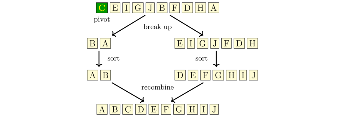
Quicksort first picks an element of the array to serve as a pivot. For simplicity, we will use the first element. Quicksort then breaks the array into the portion that consists of all the elements less than or equal to the pivot and the portion that consists of all the elements greater than the pivot. For instance, if we are sorting CEIGJBFDHA, then the pivot is C, and the two portions are BA (everything less than the pivot) and EIGJFDH (everything greater than the pivot).
We then sort the two portions using quicksort again, making this a recursive algorithm. Finally, we combine the portions. Because we know that all the things in the one portion are less than or equal to the pivot and all the things in the other portion are greater than the pivot, putting things together is quick. See the figure below:
Notice that the way quicksort breaks up the array is more complicated than the way mergesort does, but then quicksort has an easier time putting things back together than mergesort does. Here is one way to implement quicksort, coded to return a new list instead of modifying the caller's list.
def quicksort(L):
    if len(L) <= 1:
        return L[:]
    smaller = [x for x in L[1:] if x <= L[0]]
    greater = [x for x in L[1:] if x > L[0]]
    return quicksort(smaller) + [L[0]] + quicksort(greater)
This code is actually fairly slow since creating new lists in Python is a slow process. However, the code does have the benefit of being short and not too hard to understand. If we want a quick version of quicksort, we need to put more work into how to divide up the list. Instead of creating new lists, it's faster if we can do the work of dividing up the elements within L itself.
We use two indices, i and j, with i starting at the left end of the list and j starting at the right. Both indices move towards the middle of the list. We first advance i until we meet an element that is greater than or equal to the pivot. We then advance j until we meet an element that is less than or equal to the pivot. When this happens, we swap the elements at each index. We then continue advancing the indices and swapping in the same way, stopping the process once the once the i and j indices meet each other. See the figure below:
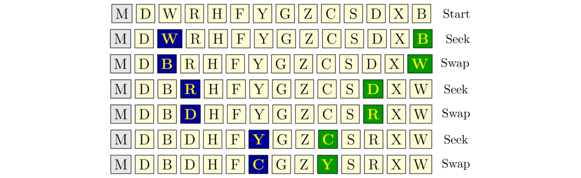
In the figure above, the pivot is M, the first letter in the list. The figure is broken down into “seek” phases, where we advance i and j, and “swap” phases, where we exchange the values at those indices. The blue highlighted letter on the left corresponds to the position of i and the green highlighted letter on the right corresponds to the position of j. Notice at the last step how they cross paths.
This process partitions the list. We then make recursive calls to quicksort, using the positions of the indices i and j to indicate where the two subarrays are located in the main array. In particular, we make a recursive call on the subarray starting at the left end and ending at the position of i, and we make a recursive call on the sublist starting at the position of j and ending at the right end. So in the example above, we would call quicksort on the sublist from 0 to 8 and from 8 to 13. Here is the code for our improved quicksort:
def quicksort(L):
    quicksort_helper(L, 0, len(L)-1)

def quicksort_helper(L, left, right):
    if left >= right:
        return

    i, j, pivot = left, right, L[left]
    while i <= j:
        while L[i] < pivot:
            i += 1
        while L[j] > pivot:
            j -= 1
        if i <= j:
            L[i], L[j] = L[j], L[i]
            i += 1
            j -= 1

    quicksort_helper(L, i, right)
    quicksort_helper(L, left, j)
Quicksort has a O(n log n) running time in the average case. The partition process will typically split the list into two roughly equal pieces, leading to O( log n) total partitions, and the partitioning process itself takes O(n) time. However, there are some special cases where it degenerates to O(n2), specifically when the list doesn't get split very equally.
One of these cases would be if the list was already sorted. Since the pivot is the first item, which is the smallest thing in the list, there will be nothing less than the pivot. So one of the recursive cases will be empty and the other will have n–1. When we call quicksort recursively on that, we will again have the same problem, with nothing less than the pivot and n–2 things greater. Things will continue this way, leading to n recursive calls, each taking O(n) time, so we end up with an O(n2) running time overall. Since real-life lists are often sorted or nearly so, this is an important problem.
One way around this problem is to use a different pivot, such as one in the middle of the list or one that is chosen randomly. Another approach is to shuffle the list once at the start before beginning the quicksort algorithm. In theory a O(n2) worst case could happen with the shuffled list, but it would be extremely unlikely.
Counting sort, bucket sorting, and radix sort
Counting sort works by keeping an array of counts of how many times each element occurs in the array. We scan through the array and each time we meet an element, we add 1 to its count. Suppose we know that our arrays will only contain integers between 0 and 9. If we have the array [1,2,5,0,1,5,1,3,5], the array of counts would be [1,3,1,1,0,3,0,0,0,0] because we have 1 zero, 3 ones, 1 two, 1 three, no fours, 3 fives, and no sixes, sevens, eights, or nines.
We can then use this array of counts to construct the sorted list [0,1,1,1,2,3,5,5,5] by repeating 0 one time, repeating 1 three times, repeating 2 one time, etc., starting from 0 and repeating each element according to its count. Here is code for the counting sort. Instead of modifying the caller's list, it returns a copy, since it's easier to code that way.
def counting_sort(L):
    # create list of counts
    counts = [0]*(max(L)+1)
    for x in L:
        counts[x] += 1

    # use counts to create sorted list
    R = []
    for i in range(len(counts)):
        R += [i]*counts[i]
    return R
The first loop of the code runs in O(n) time, as does the second, so overall, it's O(n). The only real problem here is that this sort is limited to integers in a restricted range. If L=[1000000000000, 1] this code would take a really long time to run. However, many real life lists are more reasonable than this, and counting sort would be a good approach for them. Counting sort can be made to work for some other types of data in restricted ranges.
M bucket would be pretty large. We could break it into smaller buckets, like an MA bucket, and ME bucket, etc., for all the possible first two letter combinations.
Below is a simple bucket sort for nonnegative integers. It puts the integers into 1000 different buckets based on how large the largest item in the list is. If the largest item in the list is 4999, then the first bucket is for the range from 0 to 4, the second is 5 to 9, the third is 10 to 14, etc. This comes from there being 5000 numbers and 1000 buckets. Here is the code.
    buckets = [[] for i in range(1000)]
    m = max(L) + 1
    for x in L:
        buckets[1000 * x // m].append(x)
    for B in buckets:
        insertion_sort(B)
    return [b for B in buckets for b in B]
Notice the overall approach: we create the buckets, put each list item into the appropriate bucket, sort each bucket, and then combine the buckets back into a single list. This is quite similar to counting sort, which itself is actually a type of bucket sort. If the hash function splits things up relatively evenly across the buckets, then bucket sorting has O(n) running time.
def radix_sort(L):
    for d in range(len(str(max(L)))):
        buckets = [[] for i in range(10)]
        for x in L:
            buckets[(x//10**d)%10].append(x)
        L = [b for B in buckets for b in B]
    return L
In the code above, we use len(str(max(L))) to quickly get the number of digits in the largest number in the list. This tells us how many total iterations we will have to do. At each iteration, we break the list into 10 buckets based on the current digit we are looking at. We use a little math to get that digit from each number. Namely, for the dth digit from the right of x we use (x//10**d). The second-to-last line collapses (or flattens) the list of buckets into a single list. This list is now sorted by the dth digit. When we move on to sort by the d+1st digit at the next step, that sorting will not change the order of things in the list that have the same dth digit. That's what makes this work.
Radix sort runs in O(n) time, specifically O(n log m) time, where m is the maximum element of the list. Radix sort can be modified to work with strings and other data types.
A few other sorts
Below is some Python code implementing heapsort. It uses heap operations in Python's heapq library. The heapify function turns a list into a heap. The heappop operation pops the top thing off the heap, which is always the minimum. So popping things off a heap one-by-one and adding them to a list results in a sorted list.
def heapsort(L):
    H = L[:]
    heapify(H)
    for i in range(len(L)):
        L[i] = heappop(H)
Internally, the heapify function loops over all the elements of the list and adds them one-by-one to a heap. The loop takes n steps and adding each item to the heap takes on average log n steps, so this is O(n log n) overall. The loop where we pop the items and add them to the list is O(n log n) for similar reasons.
def bogosort(L):
    while True:
        shuffle(L)
        for i in range(len(L)-1):
            if L[i+1] < L[i]:
                break
        else:
            return
The running time of this algorithm is O(n!). The notation n! is for the factorial of n, which is where we multiply all the values from n down to 1. For instance, 5! is 5 · 4 · 3 · 2 · 1 = 120. Factorials grow really fast. For instance, 10! is 3,628,800, 20! is 2,432,902,008,176,640,000, and 100! is a number that is 158 digits long. If there are n items in the list, a basic result from combinatorics or discrete math is that there are n! ways to rearrange the items (these are called permutations), and on average it will take n!/2 shuffles before we get one that works. It's worth trying bogosort out yourself with a few different lists to see how slow it really is.
def slow_sort(L):
    for i in range(len(L)):
        for j in range(i+1, len(L)):
            if L[i] > L[j]:
                L[i], L[j] = L[j], L[i]
def bubble_sort(L):
    for i in range(len(L)-1):
        for j in range(len(L)-1,i,-1):
            if L[j-1] > L[j]:
                L[j-1], L[j] = L[j], L[j-1]
Summary and running times
Overall, a sorting algorithm has to at least look at every element once, so the minimum running time for a sorting algorithm is O(n). As we've seen, counting sort and radix sort can achieve this for certain types of data. A general sorting algorithm that works for any type of data will need to do comparisons, checking to see if certain elements are greater or less than others. Any sorting algorithm that does comparisons is Omega(n log n). That is, we can't do any better than n log n. To see why, think about it this way: there are n! ways to reorder the list, and only one of those is in sorted order. If we were to do a binary search through these n! reorderings, it would take O( log(n!)) steps. If we approximate n! by nn, this becomes O( log(nn)), which simplifies to O(n log n), using properties of logarithms.
Which search to use will depend on a few factors. If the list is small, most of the sorts we covered would be fine unless speed is really important. If speed really matters, then insertion sort is good for lists of up to maybe a few dozen elements, and for anything larger, quicksort and mergesort (especially its Timsort variation) are good. Those sorts are good general purpose sorts that work with any sortable data type. But if you have very specific data in mind, like if you have a list of English words or a list of integers in the range from 1 to 10000, then counting sort, radix sort, or some type of bucket sort will likely be a better approach.
Another consideration is if the sort is stable. If you are sorting a list of objects based on a certain field, and the are multiple objects with equal values in that field, a stable sort will keep those objects in the same order as in the original list. In some situations, this is important. For instance, if we are sorting a list of person objects by age, and the objects are initially in alphabetical order by name, a stable sort will preserve that alphabetical order in that people with the same age will still be in alphabetical order. A sort that is not stable could jumble things. The standard implementations of mergesort and insertion sort are stable, while quicksort and heapsort are not. However, each of these can be modified to make them stable if needed.
A really nice audio/video demonstrating most of the sorts in this set of notes, as well as a few others, is “15 Sorting Algorithms in 6 Minutes” at https://www.youtube.com/watch?v=kPRA0W1kECg.