Spanning Trees
A weighted graph is a graph where we label each edge with a number, called its weight, like shown below.
Weighted graphs are useful for modeling many problems. The weight often represents the “cost” of using that edge. For example, the graph below might represent a road network, where the vertices are cities and the edges are roads that can be built between the cities. The weights could represent the costs of building those roads.

There are many ways to represent the weights in a graph. The one we will go with here is to use a dictionary to hold the weights of each edge. The keys of the dictionary are tuples (u,v) that represent the edge by its endpoints; the values of the dictionary are the weights.
So if a graph G has vertices called 'a' and 'b', we would get the weight by doing G.weight[('a', 'b')]. Here is the weighted graph class:
class WeightedGraph(dict):
    def __init__(self):
        self.weight = {}

    def add(self, v):
        self[v] = set()

    def add_edge(self, weight, u, v):
        self[u].add(v)
        self[v].add(u)
        self.weight[(u,v)] = self.weight[(v,u)] = weight
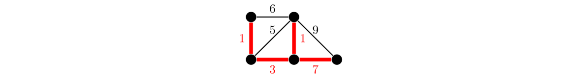
Going back to the graph above representing a road network, suppose we want to build enough roads to make it possible to get from any city to any other, and we want to do so as cheaply as possible. The answer is shown below.
When solving this problem, since we are trying to do things as cheaply as possible, we don't want any cycles, as that would mean we have a redundant edge. And we want to be able to get to any vertex in the graph, so what we want is a minimum spanning tree, a subgraph that reaches all the vertices, contains no cycles, and where the sum of all the edge weights is as small as possible. There are several algorithms for finding minimum spanning trees. We will look at two: Prim's algorithm and Kruskal's algorithm.
Prim's algorithm
Here is how it works: We pick any vertex to start from and choose the cheapest edge incident on that vertex. The tree we are building now has two vertices. Look at all the edges from these two vertices to other vertices, and pick the cheapest one. We have now added three vertices to our tree. Keep this process up, always following this rule:
Add the cheapest edge from a vertex already added to one not yet reached.
We can break edge-weight ties however we like. We stop the algorithm once every vertex has been added to the tree. Here is an example. We will start building the tree from the upper left.
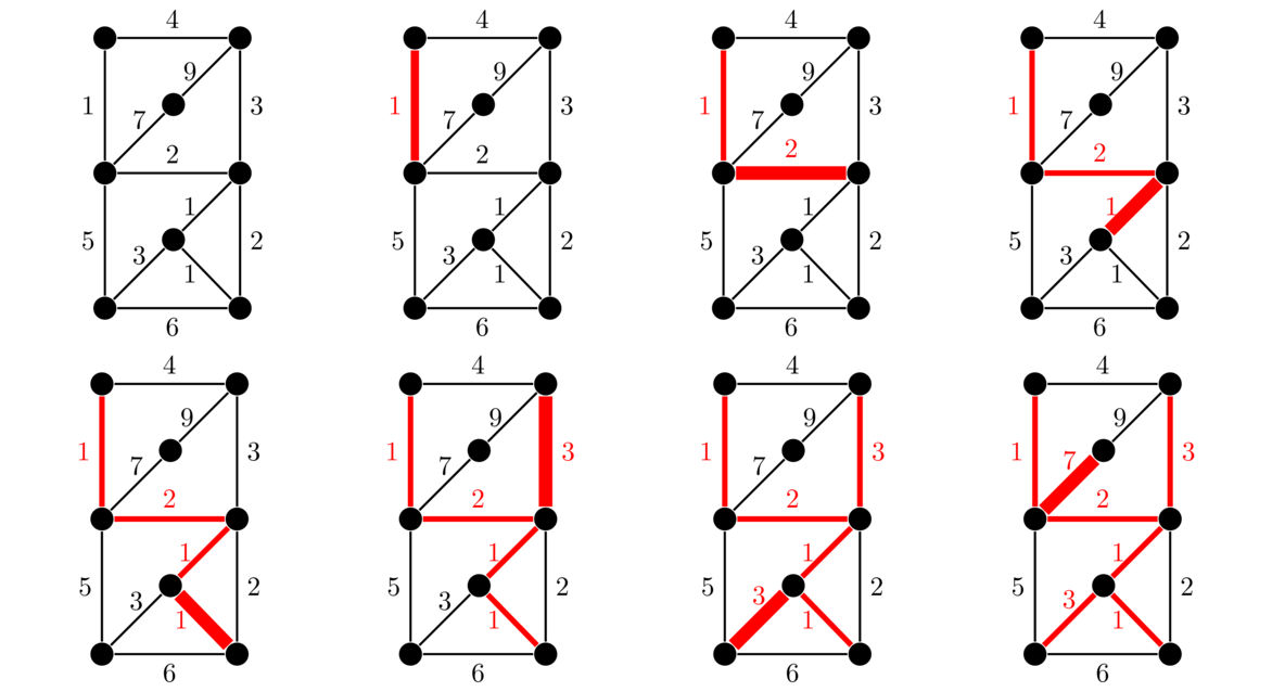
Prim's algorithm is an example of a greedy algorithm. It is called that because at each step it chooses the cheapest available edge without thinking about the future consequences of that choice. It is remarkable that this strategy will always give a minimum spanning tree.
Coding Prim's algorithm
The basic idea of Prim's algorithm is that we build up the spanning tree by always adding the cheapest edge from an already-added vertex to one that has not yet been added. To find the cheapest edge quickly, we use a heap. Specifically, whenever we add a new vertex, we add all the edges from it into the heap. This makes it quick to find the cheapest edge.
The heappush and heappop operations used below are found in Python's heapq library. Below is the code. It is very similar to the BFS code, the main difference being the use of a heap instead of a queue.
def prim(G, start):
    mst = []
    found = set()
    waiting = [(0, None, start)]

    while waiting:
        _, u, v = heappop(waiting)
        if v not in found:
            mst.append((u,v))
            if len(mst) == len(G):
                return mst[1:]
            found.add(v)
            for w in G[v]:
                heappush(waiting, (G.weight[(v,w)], v, w))

    return []
The graph passed to the function is a weighted graph. The function returns the spanning tree as a set of edges. There is not really too much happening above. We start by adding a single “edge” onto the heap. It's not really an edge, but just something to get the ball rolling from the start vertex. We then loop, continually popping things from the heap. We continue until there are len(G)-1 edges added to the spanning tree. A general fact about trees is that they will always have one less edge than the number of vertices, and we make use of that here. If the heap ever empties out before this, then the graph must not be connected and a spanning tree doesn't exist. The algorithm actually finds a spanning tree for the component of the starting vertex, though here we just return an empty list if this occurs.
The main part of the loop pops off an edge from the heap and checks to see if it is an edge to a new vertex. If it is, then we add the edge to the spanning tree, mark the new vertex as found, and add all the edges from it into the heap.
Kruskal's algorithm
Kruskal's algorithm is another approach to finding a minimum spanning tree. It is greedy, like Prim's, but it differs in how it chooses its edges. Kruskal's algorithm builds up a spanning tree of a graph G one edge at a time. The key idea is this:
At each step of the algorithm, we take the edge of G with the smallest weight such that adding that edge into the tree we are building does not create a cycle.
We can break edge-weight ties however we want. We continue adding edges according to the rule above until it is no longer possible. In a graph with n vertices, we will always need to add exactly n–1 edges. An example is shown below. Edges are highlighted in the order they are added.
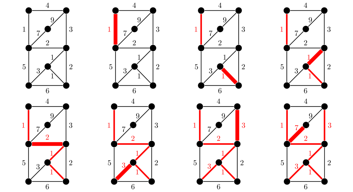
Prim's algorithm builds up a graph that is a tree at every step. Kruskal's is different in that the graph produced is disconnected up until the final step. The two algorithms might produce the same spanning tree, but they don't always. However, if the edge weights are all different, then the two algorithms will always produce the same tree.
In coding Kruskal's algorithm, we have two things to do: (1) choose the cheapest edge and (2) see if it creates a cycle. The first thing is pretty quick to do just by sorting the edges. The second thing can be done in a few ways. A simple, but slow, way is to use a BFS or DFS to see if the new edge causes a cycle.
We will instead look at a fast approach using something called the union-find data structure, which is also called the disjoint set data structure. It will take a little work to build our way up to it. We'll use the graph below in describing how the algorithm works.

We think of the spanning tree we are creating as initially starting with only vertices, and gradually we add edges. The data structure we are using is sometimes called a disjoint set data structure because it uses sets to represent the components of the graph that we build up. Initially, we have one set for each vertex, like below:
{a} {b} {c} {d} {e} {f}
Each time we add an edge between two vertices, we combine (or union) their sets together. Here are the next several steps, corresponding to adding the cheapest available edges:
add ab {a, b} {c} {d} {e}, {f}
add ef {a, b} {c} {d} {e, f}
add cf {a, b} {d} {c, e, f}
add be {a, b, c, e, f} {d}
The next edge to add would be be. But looking at the sets, we see that b and e are in the same set/component. That means its possible to get from b to e, and if we add edge be, that would give two ways to get from b to e, giving us a cycle. So we don't add be. In general, this is how we detect if there is a cycle. If the two endpoints belong to the same set, then adding that edge would create a cycle. Otherwise, we're okay. The final step for this graph would be to add edge ad, which would give us a single set containing all the vertices, and that completes the algorithm.
We could code this in a straightforward way by creating sets, but the unioning operation is slow. We can do better if instead of creating actual sets, we use a tabular approach to represent the sets. One way to do this would be to pick a specific vertex from each component to act as a representative for that set. For instance, a hypothetical table for the sets {a, b, e, f}, {c, d}, and {g}, our table might look like below.
| a | b | c | d | e | f | g |
| a | a | c | c | a | a | g |
The last piece of the puzzle is that when we union two sets, we want to keep it so that the pointer chains don't get too long. We do this by keeping a value called the rank of each vertex. When edge xy is added between two vertices of the different ranks, we trace back the pointers to find the representatives of the sets for x and y. We look at the ranks of those two representatives. If they are equal, we choose one of them (either one is okay) and increase its rank by 1. If the ranks are not equal, then we leave them be. Finally, we point the lesser-ranked representative at the larger-ranked representative.
To summarize, the union-find/disjoint set data structure uses sets to represent the components of the spanning tree being built up. When adding an edge, we first check to makes sure the two endpoints are in separate sets. If so, then we union the those two sets together. Keeping track of the sets using actual sets is inefficient, so we use a tabular approach of pointers and ranks, using specific vertices to represent each set. Each vertex starts off pointing to itself and each rank starts as 0. Every time we try to add an edge xy we do the following process:
- Trace back the pointers to find the representative of the set containing x. We do this by looking at the table entry for x, then looking at the table entry for that result, etc. until we get to an entry that points to itself. That entry is the representative of the set containing x. We also do the same process for y. This is the find portion of the union-find algorithm.
- If the representatives found in Step 1 are equal, then adding ab would cause a cycle. Go back to Step 1 and try the next cheapest available edge. Otherwise, move to Step 3.
- If the ranks of the two representatives found in Step 1 are equal, pick one of them arbitrarily and increase its rank by 1. This is the only time a rank will ever change.
- Set the pointer table entry of the lesser-ranked representative to be the higher-ranked representative (i.e. we point the lesser to the greater).
Note: One important optimization to this process happens in Step 1. Once we're done tracing back through the pointers, we go and set each of the entries to point directly to the representative. This is called path compression, and it has the effect of shrinking some of the paths, making future find operations run more quickly.
Below is an example showing how the pointers and ranks evolve. When breaking ties, we will choose the vertex that comes first alphabetically. We will also not worry about path compression. Below the graph are the order the edges are added, the tables of pointers and ranks, and what the disjoint sets look like at each step. The underlined entries in the table show values that have changed, and the underlined entries in the sets show the representative of the set.


We begin the process by adding the cheapest edge, ab. At this point, a and b both point to each other, so the find operation is simple. They both have the same rank, so we increase the rank of one of them by 1. We choose a according to our rule about breaking ties alphabetically. We then point b at a by changing its table entry to a. This is all recorded in the “add ab” row of the tables above.
The next cheapest edge is ef. This behaves very similarly to above. Here we increase the rank of e by 1 and point f at e. Next we add edge cf. Here c points to itself and f points to e. We compare the ranks of c and e and see that e is larger, so we will point c at e. The ranks don't change since they are not equal.
Next we add be. We see that b points to a and e points to itself. The ranks of both a and e are 1, so one of their ranks will increase. Breaking this tie alphabetically, we will increase the rank of a by 1 and point e at a. We then try to add edge ae, since it's the next cheapest. This isn't recorded in the tables above. The reason is that both a and e point to the same thing, meaning they are in the same set. Adding ae would cause a cycle. So we move on and look at ad. Each points to itself and the rank of a is larger, so we point d at a and don't change any ranks. And now we are done since all the vertices are part of the same set (or more simply since we have added 5 edges in a 6-vertex graph).
| a | b | c | d | e | f |
| b | b | a | c | c | f |
| a | b | c | d | e | f |
| 0 | 2 | 1 | 0 | 0 | 0 |
In the examples thus far, we haven't talked about path compression. What path compression does is when we trace back the pointers, like d → c → a → b, after we're done, we go through and set all of those to the final representative, b. This makes it so that future lookups involving these vertices will be faster since we won't have to follow as long a trail of pointers. So the pointer table will end up with a, b, c, and d all pointing to b. Note that the entry for e doesn't change here, even though it eventually points to b as well. We only perform path compression on the vertices we find while tracing back through a trail of pointers.
Coding Kruskal's algorithm
Below is the code for Kruskal's algorithm. It will be explained below.
def kruskal(G):
    mst = []
    edges = []
    for v in G:
        for w in G[v]:
            if (w, v) not in edges:
                edges.append((v,w))
    edges.sort(key = lambda e:G.weight[(e[0],e[1])])

    P = {v:v for v in G}
    R = {v:0 for v in G}

    for v, w in edges:
        rv = find(P, v)
        rw = find(P, w)
        if rv != rw:
            mst.append((v, w))
            if len(mst) == len(G) - 1:
                return mst
            union(P, R, rv, rw)
    return []   # no MST. Graph is disconnected

def find(P, v):
    L = [v]
    while v != P[v]:
        v = P[v]
        L.append(v)
    for x in L:
        P[x] = v
    return v

def union(P, R, rv, rw):
    if R[rv] == R[rw]:
        R[rv] += 1
    if R[rw] < R[rv]:
        P[rw] = rv
    else:
        P[rv] = rw
The kruskal function returns a list of the edges of the minimum spanning tree. The function first creates a list of edges and sorts them by weight. It then creates dictionaries P and R to hold the pointers and ranks of each vertex.
We loop over the sorted edges, and for each edge vw, we call the find method to find the representatives for the sets containing v and w. If they are not equal, then adding the edge won't cause a cycle, so we go ahead and add the edge to the minimum spanning tree. A basic fact from graph theory is that any tree with n vertices must have exactly n–1 edges, and we use this in the code above to determine when to exit the function. If we're not done, then we call the union function to put the two sets together (i.e. update the rank and pointer tables).
The key part of the find method is while v != P[v]: v = P[v]. This starts at the given vertex v and traces the pointers back until it gets to a vertex that points to itself. At that point it has found the representative. We could exit here, but instead we perform path compression to set all the vertices we found along the way to point to the representative. This cuts down on amount of time future searches will take since the paths to the representative will now be shorter. The union method updates the ranks and pointers, as described earlier. It breaks the tie by picking rv as the representative whose rank increases.
A few notes about spanning trees and the union-find data structure
Spanning trees have a number of applications. One use is avoiding routing loops in networks. These happen when a packet in a network keeps bouncing around between the same couple of routers instead of getting to its destination. Something called the spanning tree protocol is used by the routers to find a spanning tree in the graph created by the routers and their connections. A few other well-known applications are an algorithm to generate mazes and finding approximate solutions to the traveling salesman problem.
The union-find data structure is useful for a variety of things. It gives a faster algorithm than BFS/DFS for determining if two vertices in a graph are connected. It is also used to determine in programming languages if two variables reference the same object.
We referred to Kruskal's and Prim's algorithms as greedy algorithms. A greedy algorithm at each step always chooses the option that looks the best at that step, without consider the consequences of that choice on future steps. For instance, Kruskal's and Prim's algorithms always choose the cheapest edge they can. This type of strategy doesn't work for all problems. For instance, it would be a pretty bad way to play chess, to only look at the current turn and not consider its effect on future turns. However, greedy algorithms do give the optimal solution to a number of problems, and even when they don't, they often give a reasonably good solution quickly.