An Intuitive Introduction to Data Structures

Version 2.0
© 2019 Brian Heinold
Licensed under a Creative Commons Attribution-Noncommercial-Share Alike 4.0 Unported License

Preface

This book covers standard topics in data structures including running time analysis, dynamic arrays, linked lists, stacks, queues, recursion, binary trees, binary search trees, heaps, hashing, sets, maps, graphs, and sorting. It is based on Data Structures and Algorithms classes I've taught over the years. The first time I taught the course, I used a bunch of data structures and introductory programming books as reference, and while I liked parts of all the books, none of them approached things quite in the way I wanted, so I decided to write my own book. I originally wrote this book in 2012. This version is substantially revised and reorganized from that earlier version. My approach to topics is a lot more intuitive than it is formal. If you are looking for a formal approach, there are many books out there that take that approach.

I've tried to keep explanations short and to the point. When I was learning this material, I found that just reading about a data structure wasn't helping the material to stick, so I would instead try to implement the data structure myself. By doing that, I was really able to get a sense for how things work. This book contains many implementations of data structures, but it is recommended that you either try to implement the data structures yourself or work along with the examples in the book.

There are a few hundred exercises. They are all grouped together in Chapter 12. It is highly recommended that you do some of the exercises in order to become comfortable with the data structures and to get better at programming.

If you spot any errors, please send me a note at heinold@msmary.edu.

Running times of algorithms

Introduction

In computer science, a useful skill is to be able to look at an algorithm and predict roughly how fast it will run. Choosing the right algorithm for the job can make the difference between having something that takes a few seconds to run versus something that takes days or weeks. As an example, here are three different ways to sum up the integers from 1 to n.

Probably the most obvious way would be to loop from 1 to n and use a variable to keep a running total.
```
long total = 0;
for (long i=1; i<=n; i++)
    total += i;
```
If you know enough math, there is a formula 1+2+… +n =n(n+1)/2. So the sum could be done in one line, like below:
```
long total = n*(n+1)/2;
```

Here is a bit of a contrived approach using nested loops.

long total = 0;
for (long i=1; i<=n; i++)
    for (long j=0; j<i; j++)
        total++;

Any of these algorithms would work fine if we are just adding up numbers from 1 to 100. But if we are adding up numbers from 1 to a billion, then the choice of algorithm would really matter. On my system, I tested out adding integers from 1 to a billion. The first algorithm took about 1 second to add up everything. The next algorithm returned the answer almost instantly. I estimate the last algorithm would take around 12 years to finish, based on its progress over the three minutes I ran it.

In the terminology of computer science, the first algorithm is an O(n) algorithm, the second is an O(1) algorithm, and the third is an O(n²) algorithm.

This notation, called big O notation, is used to measure the running time of algorithms. Big O notation doesn't give the exact running time, but rather it's an order of magnitude estimation. Measuring the exact running time of an algorithm isn't practical as so many different things like processor speed, amount of memory, what else is running on the machine, the version of the programming language, etc. can affect the running time. So instead, we use big O notation, which measures how an algorithm's running time grows as some parameter n grows. In the example above, n is the integer we are summing up to, but in other cases it might be the size of an array or list, the number of items in a matrix, etc.

With big O, we usually only care about the dominant or most important term. So something like O(n²+n+1) is the same as O(n²), as n and 1 are small in comparison to n² as n grows. Also, we usually ignore constants. So O(3.47n) is the same as O(n). And if we have something like O(2n+4n³+.6n²-1), we would just write that as O(n³). Remember that big O is just an order of magnitude estimation, and we don't often care about being exact.

Estimating the running times of algorithms

To estimate the big O running time of an algorithm, here are a couple of rules of thumb:

If an algorithm runs in the same amount of time regardless of how large n is, then it is O(1).
A loop that runs n times will contributes a factor of n to the big O running time.
If loops are nested, multiply their running times.
If one loop follows another, add their running times.
If the loop variable is increasing in a way such as i=i*2 or i=i/3, instead of changing by a constant amount (like i++ or i-=2), then that contributes a factor of log n to the big O running time.

Here are several examples of how to compute the big O running time of some code segments. All of these involve working with an array, and we will assume n is the length of the array.

Here is code that sums up the entries in an array:
```
int total = 0;
for (int i=0; i<a.length; i++)
    total += a[i];
```
This code runs in O(n) time. It is a pretty ordinary loop.
Here is some code involving nested for loops:
```
for (int i=0; i<a.length; i++)
    for (int j=0; j<a.length; j++)
        System.out.println(a[i]+a[j]);
```
These are two pretty ordinary loops, each running for n= a.length steps. They are nested, so their running times multiply, and overall the running time is O(n²). For each of the n times the outer loop runs, the inner loop has to also run n times, which is where the n² comes from.
Here are three nested loops:
```
for (int i=0; i<a.length; i++)
    for (int j=0; j<a.length-1; j++)
        for (int k=0; k<a.length-2; k++)
            System.out.println(a[i]+a[j]*a[k]);
```
This code runs in O(n³) time. Technically, since the second and third loops don't run the full length of the array, we could write it as O(n(n-1)(n-2)), but remember that we are only interested in the most important term, which is n³, as n(n-1)(n-2) can be written as n³ plus a few smaller terms.
Here are two loops, one after another:
```
int count=0, count2=0;
for (int i=0; i<a.length; i++)
    count++;

for (int i=0; i<a.length; i++)
    count2+=2;
```
The running time here is O(n+n)=O(2n), which we simplify to O(n) because we ignore constants.
Here are a few simple lines of code:
```
int w = a[0];
int z = a[a.length-1];
System.out.println(w + z);
```
The running time here is O(1). The key idea is that the running time has no dependence on n. No matter how large that array is, this code will always take the same amount of time to run.
Here is some code with a loop:
```
int c = 0;
int stop = 100;
for (int i=0; i<stop; i++)
    c += a[i];
```
Despite the loop, this code runs in O(1) time. The loop always runs to 100, regardless of how large the array is. Notice that a.length never appears in the code.
Here is a different kind of loop:
```
int sum = 0;
for (int i=1; i<a.length; i *= 2)
    sum += a[i];
```
This code runs in O(log n) time. The reason is the that the loop variable is increasing via i *= 2. It goes up as 1, 2, 4, 8, 16, 32, 64, 128, …. It takes only 10 steps to get to 1000, 20 steps to get to 1 million, and 30 steps to get to 1 billion.
The number of steps to get to n is gotten by solving 2^x = n, and the solution to that is log₂(n) (which we often write just as log(n)).^**For logs, there is a formula, called the change-of-base-formula, that says log_a(x)=log_b(x)/log_b(a). In particular, all logs are constant multiples of each other, and with big O, we don't care about constants. So we can just write O(log n) and say that the running time is logarithmic.
Here is a set of nested loops:
```
n = a.length;
for (int i=0; i<n; i++) {
    sum = 0;
    int m = n;
    while (m > 1) {
        sum += m;
        m /= 2;
    }
}    
```
This code has running time O(n log n). The outer loop is a pretty ordinary one and contributes the factor of n to the running time. The inner loop is a logarithmic one as the loop variable is cut in half at each stage. Since the loops are nested, we multiply their running times to get O(n log n).
Here is some code with several loops:
```
total = 0;
int i=0;
while (i<a.length) {
    i++;
    total += a[i];
}

for (int i=0; i<a.length/2; i++)
    for (int j=a.length-1; j>=0 j--)
        total += a[i]*a[j];
```
The running time is O(n²). To get this, start with the fact that the while loop runs in O(n) time. The nested loops' running times multiply to give O(n · n/2). The while loop and the nested loops follow one another, so we add their running times to get O(n+n · n/2). But remember that we only care about the dominant term, and we drop constants, so the end result is O(n²).

Common running times

The most common running times are probably O(1), O(log n), O(n), O(n log n), O(n²), and O(2ⁿ). These are listed in order of desirability. An O(1) algorithm is usually the most preferable, while an O(2ⁿ) algorithm should be avoided if at all possible.

To get a good feel for the functions, it helps to compare them side by side. The table below compares the values of several common functions for varying values of n.

	1	10	100	1000	10000
1	1	1	1	1	1
log n	0	3.3	6.6	10.0	13.3
n	1	10	100	1000	10,000
n log n	0	33	664	9966	132,877
n²	1	100	10,000	1,000,000	100,000,000
2ⁿ	2	1024	1.2× 10³⁰	1.1× 10³⁰¹	2.0× 10³⁰¹⁰

Things to note:

The first line remains constant. This is why O(1) algorithms are usually preferable. No matter how large the input gets, the running time stays the same.
Logarithmic growth is extremely slow. An O(log n) algorithm is often nearly as good as an O(1) algorithm. Each increase by a factor of 10 in n only corresponds to a growth of about 3.3 in the logarithm. Even at the incredibly large value n=10¹⁰⁰ (1 followed by 100 zeros), log n is only about 332.
Linear growth (O(n)) is what we are most familiar with from real life. If we double the input size, we double the running time. If we increase the input size by a factor of 10, the running time also increases by a factor of 10. This kind of growth is often manageable. A lot of important algorithms can't be done in O(1) or O(log n) time, so it's nice to be able to find a linear algorithm in those cases.
The next line, for n log n, is sometimes called loglinear or linarithmic growth. It is worse than O(n), but not all that much worse. The most common occurrence of this kind of growth is in the running times of the best sorting algorithms.
With quadratic growth (O(n²)), things start to go off the rails a bit. We can see already with n=10,000 that n² is 100 million. Whereas with linear growth, doubling the input size doubles the running time, with quadratic growth, doubling the input size corresponds to increasing the running time by 4 times (since 4=2²). Increasing the input size by a factor of 10 corresponds to increasing the running time by 10²=100 times. Some problems by their very nature are O(n²), like adding up the elements in a 2-dimensional array. But in other cases, with some thought, an O(n²) algorithm can be replaced with an O(n) algorithm. If it's possible that the n you're dealing with could get large, it is worth the time to try to find a replacement for an O(n²) algorithm.
The last line is exponential growth, O(2ⁿ). Exponential growth gets out of hand extremely quickly. None of the examples we saw earlier had this running time, but there are a number of important practical optimization problems whose best known running times are exponential.
Other running times — There are infinitely many other running times, like O(n³), O(n⁴), …, or O(n^1.5), O(n!), and O(2^2ⁿ). The ones listed above are just the most common.

Some notes about big O notation

Here are a few important notes about big O notation.

When we measure running times of algorithms, we can consider the best-case, worst-case, and average-case performance. For instance, let's say we are searching an array element-by-element to find the location of a particular item. The best case would be if the item we are looking for is the first thing in the list. That's an O(1) running time. The worst case is if the element is the last thing, corresponding to a O(n) running time. The average case is that we will need to search around half of the elements before finding the element, corresponding to a O(n/2) running time, which we would write as O(n), since we ignore constants with big O notation. Of the three, usually what we will refer to when looking at the big O of an algorithm is the worst case running time. Best case is interesting, but not often all that useful. Average case is probably the most useful, but often it is harder to find than the worst case, and often it turns out to have the same big O as the worst case.
We have mostly ignored constants, referring to values such as 3n, 4n, and 5n all as O(n). Often this is fine, but in a lot of practical scenarios this won't give the whole story. For instance, consider algorithm A that has an exact running time of 10000n seconds and algorithm B that has an exact running time of .001n² seconds. Then A is O(n) and B is O(n²). Suppose for whatever problem these algorithms are used to solve that n tends to be around 100. Then algorithm A will take around 1,000,000 seconds to run, while algorithm B will take 10 seconds. So the quadratic algorithm is clearly better here. However, once n gets sufficiently large (in this case around 10 million), then algorithm A begins to be better. An O(n) algorithm will always eventually have a faster running time than any O(n²) algorithm, but n might have to be very large before that happens. And that value of n might turn out larger than anything that comes up in real situations. Big O notation is sometimes called the asymptotic running time, in that it's sort of what you get as you let n tend toward infinity, like you would to find an asymptote. Often this is a useful measure of running time, but sometimes it isn't.
Big O is used for more than just running times. It is also used to measure how much space or memory an algorithm requires. For example, one way to reverse an array is to create a new array, run through the original in reverse order, and fill up the new array. This uses O(n) space, as we need to create a new array of the same size as the original. Another way to reverse an array consists of swapping the first and last elements, the second and second-to-last elements, etc. This requires only one additional variable that is used in the swapping process. So this algorithm uses O(1) space. There is often a tradeoff where you can speed up an algorithm by using more space or save space at the cost of slowing down the algorithm.
Big O notation sometimes can have multiple parameters. For instance, if we are searching for a substring of length m inside a string of length n, we might talk about an algorithm that has running time O(n+m).
Last, but not least, we have been using big O notation somewhat incorrectly. Instead we really should be using something called big theta, as in Θ(n) instead of O(n). In formal computer science, big O is sort of a “no worse than” running time. That is, O(1) and O(n) algorithms are technically also O(n²) algorithms because a running time of 1 or n is no worse than n². Big O is sort of like a “less than or equal to”, while big theta is used for “exactly equal to”. However, most people are not really careful about this and use big O when technically they should use big theta. We will do the same thing here. If you are around someone pedantic or if you take a more advanced course in algorithms, then you might want to use big theta, but otherwise big O is fine.

Logarithms and Binary Search

Here is a common way of searching through an array to determine if it contains a particular item:

public static boolean linearSearch(int[] a, int item) {
    for (int i=0; i<a.length; i++)
        if (a[i]==item)
            return true;
    return false;
}

This is probably the most straightforward way of searching—check the first item, then the second item, etc. It is called a linear search, and its running time is O(n). However, this is not the most efficient type of search. If the data in the array is in order, then there is an O(log n) algorithm called the binary search that can be used.

To understand how it works, imagine a guess-a-number game. A person picks a random number from 1 to 1000 and you have 10 guesses to get it right. After each guess, you are told if your guess is too high or too low. Your first guess should be 500, as whether it's too high or too low, you will immediately have eliminated 500 numbers from consideration, which is the highest amount you can guarantee removing. Now let's suppose that 500 turns out to be too low. Then you know that the number is between 500 and 1000, so your next guess should be halfway between them, at 750. Suppose 750 turns out to be too high. Then you know the number is between 500 and 750, so your next guess should be 625, halfway between again.

At each step, the number of possibilities is cut in half from 1000 to 500 to 250, and so on, and after 10 of these halvings, there is only one possibility left. A binary search of an array is essentially this process. We look at the middle item of the array and compare it with the thing we are looking for. Either we get really lucky and find it, or else that middle element is either larger or smaller than what we are looking for. If it is larger, then we know to check the first half of the array, and otherwise we check the second half. Then we repeat the process just like with the guess-a-number game, until we either find the element or run out of places to look. In general, if there are n items, then no more than about log₂(n) guesses will be needed, making this an O(log n) algorithm. Here is the code for it:

public static boolean binarySearch(int[] a, int item) {
    int start=0, end=a.length-1;
    
    while(end >= start) {
        int mid = (start + end) / 2;
    
        if (a[mid] == item)
            return true;
        if (a[mid] > item)
            end = mid - 1;
        else
            start = mid + 1;
    }    
    return false;
}

Inside the loop, the code first locates the middle index^** A better approach is to use start + ((end - start) / 2) which avoids a potential overflow problem, but for clarity, we have taken the simpler approach. We then compare the middle item to the one we are looking for and adjust the start or end variables, which has the effect of focusing our attention on one half or the other of the array.

If possible, a binary search should be used over a linear search. For instance, a linear search on a list of 10 billion items will involve 10 billion checks if the item is not in the list, while a binary search will only require log₂(10 billion})= 34 checks.

However, binary search does require the data to be sorted, and the initial sort will take longer than a single linear search. So a linear search would make sense if you are only doing one search, and it would also make sense if the items in the array are of a data type that can't be sorted. A linear search would also be fine for very small arrays.

Lists

Dynamic arrays

Throughout these notes, we will look at several data structures. For each one we will show how to implement it from scratch so that we can get a sense for how it works. For many of these data structures, we will also talk about how to use the versions of them that are built in to Java. Generally, the classes we build here are for demonstration purposes only. They are so we can learn the internals of these data structures. It is recommended to use the ones built in to Java whenever possible as Java's classes have been much more carefully designed and tested.

The first data structure we will talk about is the list. A list is a collection of objects, such as [5, 31, 19, 27, 16], where order matters and there may be repeated elements. We will look at two ways to implement lists: dynamic arrays and linked lists.

Let's start out with looking at an ordinary Java array. An array is data stored in a contiguous chunk of memory, like in the figure below.

Each cell in the array has the same data type, meaning it takes up the same amount of space. This makes it quick to access any given location in the array. For instance, to access the element at index 5 in an array a in Java, we use a[5]. Internally, Java finds that location via a simple computation, which takes the starting memory location of the array and adds to it 5 times the size of the array's data type. In short, getting and setting elements in an array is a very fast O(1) operation.

The main limitation of Java's arrays is that they are fixed in size. Often we don't know up front how much space we will need. We can always just create our arrays with a million elements apiece, but that's wasteful. This brings us to the concept of dynamic arrays. A dynamic array is an array that can grow as needed to accommodate new elements. We can create this data structure using an ordinary array. We can start the array small, maybe making it 10 items long. Once we use up those 10 spots in the array, we create a new array and copy over all the stuff from the old array to the new one. Java will automatically free up the space in that old array to be used elsewhere in a process called garbage collection.

One question is how big we should make the new array. If we make it too small, then the expensive operation of copying the old array over will have to be done too often. A simple and reasonable thing to do is to make the new array double the size of the old one.

Implementing a dynamic array

Here is the start of a dynamic array class:

public class AList {
    private int[] data;
    private int numElements;
    private int capacity;
    
    public AList() {
        numElements = 0;
        capacity = 10;
        data = new int[capacity];        
    }
}

We have an array to hold the data, a variable called numElements thats keeps track of how many data values are in the list, and a variable called capacity that is the size of the data array. Once numElements reaches capacity, we will run out of room in the current array.

For instance, consider the list [77, 24, 11]. It has three elements, so numElements is 3. The capacity in the figure is 10.^**Note that capacity is always the same as data.length, so we could just use that and not have a capacity variable at all. However, I think it's a little clearer to have a separate variable.

Adding elements

To add an element, there are a few things to do. First, we need to check if the array is at capacity. If so, then we need to enlarge it. We do that by calling a separate enlarge method. In terms of actually adding the element to the array, we use the numElements variable to tell us where in the data array to add the element. Specifically, it should go right after the last data value. We also need to increase numElements by 1 after adding the new item. Here is the code:

public void add(int item) {
    if (numElements >= capacity)
        enlarge();
    data[numElements] = item;
    numElements++;
}

Below is the code that enlarges the array as needed. What we do is create a new array that is twice the size of the current one, then copy over all data from the old array into this one. After that, we update the capacity variable and point the data variable to our new array.

private void enlarge() {
    int[] copy = new int[capacity*2];
    for (int i=0; i<capacity; i++)
        copy[i] = data[i];
    capacity *= 2;
    data = copy;
}

Notice the design decision to make enlarge a private method. This is because it is part of the internal plumbing that our class uses to make things work, but it's not something that users of our class should need to see or use.^**In a real situation, maybe there could be a few cases where users might want to be able to enlarge the array themselves, though likely 99.9% of users would not ever use that feature, and some may accidentally misuse it.

Displaying the contents of the dynamic array

We now have a working dynamic array, but we don't have any way yet to see what is in it. To do that, we will write a toString method. The toString method is a special method that is designed to work with Java's printing methods. So if we create an AList object called list, then System.out.println(list) will automatically call our toString method to get a string representation of our list to print. Here is the method:

@Override
public String toString() {
    if (numElements == 0)
        return "[]";
    
    String s = "[";
    for (int i=0; i<numElements-1; i++)
        s += data[i] + ", ";
    s += data[numElements-1] + "]";
    return s;
}

It returns the items in the list with square brackets around them and commas between them. The code builds up a string one item at a time.^**It would be more efficient to use Java's StringBuilder class for this, but to keep things simple we won't do that. In order to avoid a comma being generated after the last element, we stop the loop one short of the end, and add the last element in separately. Note also the special case for an empty list.

Here is some code to test out our class. We first add a couple of elements and print out the list, and then we add enough elements to force the array to have to be enlarged, to make sure that process works.

public static void main(String[] args) {
    AList list = new AList();
    list.add(2);
    list.add(4);
    System.out.println(list);
    for (int i=0; i<10; i++)
        list.add(i);
    System.out.println(list);
}

When testing out a class like this, be sure also test out all the various edge cases you can think of. For example, if testing out a method that inserts items into a list, edge cases would be inserting at the start or end of a list or inserting into an empty list. In general, try to think of as many interesting scenarios that can give your code trouble. The extra time spent testing now can save a lot more time in the future tracking down bugs.

More methods

To make our list class more useful, there are a few other methods we might add. Some of these methods are also good for programming practice, as they demonstrate useful techniques for working with lists and arrays.

Getting and setting elements

Since the data is stored in an ordinary Java array, getting and setting elements can be done with simple array operations. Here are both methods:

public int get(int index) {
    return data[index];
}

public void set(int index, int value) {
    data[index] = value;
}

In both cases, we really should do some error-checking to make sure the index chosen is valid. Both methods should have code like the following:

if (index < 0 || index >= numElements)
    throw new RuntimeException("List index " + index + " is out of bounds.");

For the sake of simplicity, since our goal is to understand how data structures work, we will usually not do much error-checking, as real error-checking code can often become long enough to obscure how the data structure works.

Getting the size of the list

Since we have a variable keeping track of how many things are in the list, finding the size is easy:

public int size() {
    return numElements;
}

Lists often have a separate method called isEmpty that tells if the list has anything in it or not. We can do that by checking if numElements is 0 or not. A standard way to do that would involve four lines of code with an if/else statement. However, there is a slick way to do this in one line of code, shown below.

public boolean isEmpty() {
    return numElements == 0;
}

In Java, numElements==0 is a boolean expression that returns true or false. While we usually use that sort of thing inside an if statement, there is nothing stopping us from using it other places. So rather than use an if/else, we can shortcut the process by just returning the value of this expression. This is a common trick you will see when reading other people's code.

A contains method

A useful task is to see if a list contains something. We can use a linear search to do that.

public boolean contains(int value) {
    for (int i=0; i<numElements; i++)
        if (data[i] == value)
            return true;
    return false;
}

A common mistake is to have an else statement inside the loop that returns false. The problem with this is that the code checks the first item and immediately returns false if it is not the thing being searched for. In the approach above, we only return false if the code gets all the way through the loop and hasn't found the desired element.

Reversing a list

The first thing we would want to decide is if we want it to modify the list itself or return a new list. Let's say we want to modify the list. Here is one approach:

public void reverse() {
    int[] rev = new int[capacity];
    int j = 0;
    for (int i=numElements-1; i>=0; i--) {
        rev[j] = data[i];
        j++;
    }
    data = rev;
}

This is a relatively straightforward approach that loops through the data array backwards and fills up a new array with those elements and then replaces the old data array with the new one. Note that we use a separate index variable j to advance us through the new array. Here is another approach that avoids creating a new array:

public void reverse2() {
    for (int i=0; i<numElements/2; i++) {
        int hold = data[i];
        data[i] = data[numElements-1-i];
        data[numElements-1-i] = hold;
    }
}

The way this approach works is it swaps the first and last element, then it swaps the second and second-to-last elements, etc. It stops right at the middle of the list.

Note: A common mistake in writing these and other methods is to loop to capacity instead of numElements. The array's data values end at index numElements-1. Everything beyond there is essentially garbage.

Deleting things

An efficient way to delete an item from the array is to slide everything to the right of it down by one index. As each item is being slid down, it overwrites the item in that place. For an illustration, see the figure below where the element 5 is being deleted. The algorithm starts by overwriting 5 with 7, then overwriting 7 with 8, and then overwriting 8 with 9. The last item in the list is not overwritten, but by decreasing numElements by 1, we make that index essentially inaccessible to the other methods because all of our methods never look beyond index numElements-1.

Here is how we would code it:

public void delete(int index) {
    for (int i=index; i<numElements; i++)
        data[i] = data[i+1];
    numElements--;
}

Inserting things

To insert something, we shift elements over to the right to make room for the new element and then add the element. Shifting to the right is very similar to the left-shift from the delete method, except that we work through the array in the opposite order. Also, since we are adding to the list, we need to enlarge the array if we are out of room. The code is below:

public void insert(int index, int value) {
    if (numElements >= capacity)
        enlarge();
    for (int i=numElements-1; i>=index; i--)
        data[i+1] = data[i];
    data[index] = value;
    numElements++;
}

Running times

Looking back at the code we wrote, here are the big O running times of the methods.

The add method is O(1) most of the time. The enlarge method is O(n) and every once in a while the add method needs to call it.^**Computer scientists would say the running time of add() is amortized O(1) because the cost of the slow enlarge() method is spread out over all of the adds. For instance, if we call add() 1000 times in a row, the enlarge() method will be called 7 times (when the list size reaches 10, 20, 40, 80, 160, 320, and 640), but those 7 enlarge() calls, spread out over 1000 adds, average out to an O(1) running time.
The size and isEmpty methods are O(1). Each of them consists of a single operation with no loop involved. In some implementations of a list data structure, the size method would be O(n), where you would loop through the list and count how many items you see. However, since we are maintaining a variable numElements that keeps track of the size, that counting is spread out over all the calls to the add method.
The get and set methods are O(1). Each of them consists of a single operation with no loop involved.
The reverse method is O(n). The first reverse method we wrote has a single loop that runs through the entire array, so it's O(n). The second reverse method loops through half of the array, so it's O(n/2), but since we ignore constants, we say it's O(n). Still in a practical sense, the second method is about twice as fast as the first.
The contains, insert, and delete methods are all O(n). Remember that for big O, we are usually concerned with the worst case scenarios. For the contains method, this would be if the item is not in the list. For the insert and delete methods, this would be for inserting/deleting at index 0. In all these cases, we have to loop through the entire array, so we get O(n).

Linked lists

Linked lists provide a completely different approach to implementing a list data structure. With arrays, the elements are all stored next to each other, one after another, in memory. With a linked list, the elements can be spread out all over memory.

In particular, each element in a linked list is paired with a link that points to where the next element is stored in memory. So a linked list is just sort of strung along from one element to the next across memory, as in the figure below.

The linked list shown above is often drawn like this:

Each item in a linked list is called a node. Each node consists of a data value as well as a link to the next node in the list. The last node's link is null; in other words, it is a link going nowhere. This indicates the end of the list.

Implementing a linked list

Each element or node in the list is a pair of things: a data value and a link. In Java, to pair things like this, we create a class, which we will call Node. The data type of the value will be an integer. But what about the link's data type? It points to another Node object, so that's what its data type will be—a Node. So the class will contain references to itself, making it recursive in a sense. Here is the outline of the linked list class, with the Node class being a private inner class.

public class LList {
    private class Node {
        public int value;
        public Node next;
        
        public Node(int value, Node next) {
            this.value = value;
            this.next = next;
        }
    }
    
    private Node front;
    
    public LList() {
        front = null;
    }
}

The linked list class itself only has one class variable, a Node variable called front that keeps track of which node is at the front of the list. The Node class is made private since it is an internal implementation detail of the LList class, not something that users of our list need to worry about. The Node class is quite simple, having just the two class variables and a constructor that sets their values.^**Note that those variables are public. This keeps the syntax a little simpler. In Java, the convention is usually to make things private. But here our goal is learn about data structures, and using private variable with getters and setters will complicate the code, making it harder to see the essential ideas of linked lists.

Adding to the front of a linked list

Let's look first at adding to the front of a linked list. To do that, we need to do three things: create a new node, point that new node to the old front of the list, and then make the new node into the new front of the list. See the figure below.

It often helps to draw figures like this first and use them to create the linked list code. Here is code that does this process:.

Node node = new Node(value, null)
node.next = front;
front = node;

Working with linked lists often involves creating new nodes and moving links around. Below is an imaginative view of what memory might look like, with a linked list before and after adding a new item at the front.

We see that we have to first create the new node in memory. As we're creating that node, we specify what it will point to, and after that we have to move the front marker from its old location so that it's now indicating the new node is the front.

The three lines of code can actually be done in a single line, like below:

public void addToFront(int value) {
    front = new Node(value, front);
}

Adding to the back of a linked list

Since we don't have a pointer to the back of the list, like we have one pointing to the front of the list, adding to the back is a bit more work. We have to walk the list item-by-item to get to the back and then create and add a new node there. The loop that we use to walk the list has the following form:

Node node = front;
while (node.next != null)
    node = node.next;

This loop is one that is very useful for looping through linked lists. The idea of it is that we create a Node variable called node that acts as a loop variable, similar to how the variable i is used in a typical for loop. This Node variable starts at the beginning of the list via the line node = front. Then the line node = node.next moves the node variable through the list one node at a time. The loop condition node.next != null stops us just short of the last variable. A lot of times we will want to use node != null in its place to make sure we get through the whole list. In both cases, remember that the way we know when to stop the loop is that the end of the list is marked by a null link.

Here is the complete add method:

public void add(int value) {
    if (front == null)
        front = new Node(value, null);
    else {
        Node node = front;
        while (node.next != null)
            node = node.next;
        node.next = new Node(value, null);
    }
}

Note the special case at the start. Checking if front==null checks if the list is empty. In particular, when adding to an empty list, not only do we have to create a new node, but we also need to set the front variable to point to it. If we leave this code out, we would get a very common linked list error message: a null pointer exception. What would happen is if the list is empty, then node=front will set node to null. Then when we try to check node.next, we are trying to get a field from something that has no fields (it is null). That gives a null pointer exception.

The last line of code of the method creates the new node and points the old last node of the list to this new node. This is shown in the figure below.

Note also that the code that creates a new node sets its link to null. This is because the end of a list is indicated by a null link, and the node we are creating is to go at the end of the list.

toString()

This method is a lot like the toString method for dynamic arrays except that in place of the for loop that is used for dynamic arrays, we use a linked list while loop. Here is the code:

@Override
public String toString() {
    if (front == null)
        return "[]";
    String s = "[";
    Node node = front;
    while (node.next != null) {
        s += node.value + ", ";
        node = node.next;
    }
    s += node.value + "]";
    return s;
}

Now we can test out our code to make sure it is working:

public static void main(String[] args) {
    LList list = new LList();
    list.add(1);
    list.add(2);
    System.out.println(list);
}

It's worth stopping here to take stock of what we have done. Namely, we have managed to create a list essentially from scratch, without using arrays, where the array-like behavior is simulated by linking the items together.

size and isEmpty

Finding the size of a linked list gives us another opportunity to use the standard linked list loop:

public int size() {
    int count = 0;
    Node node = front;
    while (node != null) {
        count++;
        node = node.next;
    }
    return count;
}

To check if a list is empty, we need only check if the front variable points to something or if it is null. This can be done very quickly, like below:

public boolean isEmpty() {
    return front == null;
}

Getting and setting elements

Getting and setting things in a linked list is harder than for dynamic arrays. The problem is that we can't just jump right to the index we need. Instead, we have to walk through the list node-by-node until we get to the desired index. We can do that with a while loop like the ones we have been using, except that we stop the loop when we get to the desired index. Below are the two methods. They are the same except for their last lines.

public int get(int index) {
    int count = 0;
    Node node = front;
    while (count < index) {
        count++;
        node = node.next;
    }
    return node.value;
}

public void set(int index, int value) {
    int count = 0;
    Node node = front;
    while (count < index) {
        count++;
        node = node.next;
    }
    node.value = value;
}

Deleting items

To delete a node, we reroute the link of the node immediately before it as below (the middle node is being deleted).

To do this, we step through the list node-by-node, using a loop similar to the ones for the get and set methods. Once the loop variable node reaches the node immediately before the one being deleted, we use the following line to perform the deletion:

node.next = node.next.next;

This line reroute's node's link around the deleted node so it points to the node immediately after the deleted node. That deleted node is still sitting there in memory, but with nothing now pointing to it, it is no longer part of the list. Eventually Java's garbage collection algorithm will come around and allow that part of memory to be reused for other purposes.

The full delete code is below. Note that the line above will not work for deleting the first index, so we need a special case for that. To handle it, it suffices to do front = front.next, which moves the front variable to point to the second thing in the list, making that the new front.

public void delete(int index) {
    if (index == 0)
        front = front.next;
    else {
        int count = 0;
        Node node = front;
        while (count < index-1) {
            count++;
            node = node.next;
        }
        node.next = node.next.next;
    }
}

Note also that we don't need a special case for deleting the last thing in the list. Try to see why the code will work just fine in that case.

Inserting into a list

Here is a figure to help us write code for the insert method:

We can see that to insert a node, we go the node immediately before index we need. Let's call it node. We point node's link to a new node that we create, and make sure the new node's link points to what the node used to point to. The node creation and rerouting of links can be done in one line, like this:

node.next = new Node(value, node.next);

Much of the code for inserting into a list is similar to the delete method. In particular, we need a special case for inserting at the beginning of the list (where we can simply call the addToFront method that we already wrote), and the code that loops to get to the insertion point is the same as the delete method's code. Here is the method:

public void insert(int index, int value) {
    if (index == 0)
        addToFront(value);
    else {
        int count = 0;
        Node node = front;
        while (count < index-1) {
            count++;
            node = node.next;
        }
        node.next = new Node(value, node.next);
    }
}

Working with linked lists

The best way to get comfortable with linked lists is to write some linked list code. Here are a few helpful hints for working with linked lists.

Basics

First, remember the basic idea of a linked list, that each item in the list is a node that contains a data value and a link to the next node in the list. Creating a new node is done with a line like below:

Node node = new Node(19, null);

This creates a node with value 19 and a link that points to nothing. Suppose we want to create a new node that points to another node in the list called node2. Then we would do the following:

Node node = new Node(19, node2);

To change the link of node to point to something else, say the front of the list, we could do the following:

node.next = front;

Remember that the front marker is a Node variable that keeps track of which node is at the front of the list. The line below moves the front marker one spot forward in the list (essentially deleting the first element of the list):

front = front.next;

Looping

To move through a linked list, a loop like below is used:

Node node = front;
while (node != null)
    node = node.next;

This will loop through the entire list. If we use node.next != null, that will stop us at the last element instead of moving through the whole list. If we want to stop at a certain index in the list, we can use a loop like the one below (looping to index 10):

Node node = front;
int count = 0;
while (count < 10) {
    count++;
    node = node.next;
}

Using pictures

Many linked list methods just involve creating some new nodes and moving some links around. To keep everything straight, it can be helpful to draw a picture. For instance, below is the picture we used earlier when describing how to add a new node to the front of a list:

And we translated this picture into the following line:

front = new Node(value, front);

This line does a few things. It creates a new node, points that node to the old front of the list, and moves the front marker to be at this new node.

Edge cases

When working with linked lists, as with many other things, it is important to worry about edge cases. These are special cases like an empty list, a list with one element, deleting the first or last element in a list, etc. Often with linked list code, one case will handle almost everything except for one or two special edge cases that require their own code.

For instance, as we saw earlier, to delete a node from a list, we loop through the list until we get to the node right before the node to be deleted and reroute that node's link around the deleted node. But this won't work if we are deleting the first element of the list. So that's an edge case, and we need a special case to handle that.

Null pointer exceptions

When working with nodes, there is a good chance of making a mistake and getting a null pointer exception from Java. This usually happens if you use an object without first initializing it. For example, the following will cause a null pointer exception:

Node node;
// some code not involving node might go here...
if (node.value == 3)
    // some more code goes here...

Since the node variable was not initialized to anything, its current value is the special Java value, null. When we try to access node.value, we get a null pointer exception because node is null and has no field called value.

The correction is to either set node equal to some other Node object or initialize it like below:

Node node = new Node(42, null);

In summary, if you get a null pointer exception, it often indicates an object that has been declared but not initialized. It also frequently happens with a linked list loop that accidentally loops past the end of the list (which is indicated by null).

A couple of trickier examples

A doubling method

Here is a linked list method that replaces each copy of an element with two copies of itself. For instance, if the list is [1,2,3], after calling this method it will be [1,1,2,2,3,3]. Here is the code:

public void doubler() {
    Node node = front;
    while (node != null) {
        node.next = new Node(node.value, node.next);
        node = node.next.next;
    }
}

We do this with a single loop. At each step of the loop, we make a copy of the current node and point the current node to the copy. Then we move to the next node. But we can't just do node = node.next because that will move from the current node to its copy, and we will end up with an infinite loop that keeps copying the same value over and over. Instead, node = node.next.next moves us forward by two elements in the list.

Note that we could do this method by looping through the list and calling the insert method. However, that would be an O(n²) approach as the insert method itself uses a loop to get to the appropriate locations. That of course is wasteful since we are already at the appropriate location. The approach given above is O(n).

Removing zeroes

Let's write a method to remove all the zeroes from the list. We could do this by looping through the list, checking if the current element is 0, and calling the delete method, but that would be an O(n²) approach. Here is an O(n) approach:

public void removeZeros() {
    while (front != null && front.value == 0)
        front = front.next;

    Node node = front;
    while (node != null && node.next != null) {
        while (node.next != null && node.next.value == 0)
            node.next = node.next.next;
        node = node.next;
    }
}

Writing this requires some real care. First, dealing with zeroes at the start of the list is different from dealing with them in the middle. To delete a zero at the front of the array, we can use front = front.next. However, it may happen that the next element is also zero and maybe the one after that, so we use a loop. We also need to be careful that the list is not all zeroes, as we can easily end up with a null pointer exception that way. The first two lines of the method take care of all of this.

The next few lines handle zeroes in the middle of the array. We can delete these zeroes by rerouting links in the same way that the delete method does. But we have to be careful about multiple zeroes in a row. To handle this, every time we see a zero, we loop until we stop seeing zeroes or reach the end of the list. Note that despite the nested loops, they both affect the loop variable node, so overall this is still an O(n) algorithm.

To test this method out, try it with a variety of cases including lists of all zeroes, lists that start with multiple zeroes, lists that end with multiple zeroes, and various other combinations.

Making the linked list class generic

The linked list class we created works only with integer data. We could modify it to work with strings by going through and replacing the int declarations with String declarations, but that would be tedious. And then if we wanted to modify it to work with doubles or longs or some object, we would have to do the same tedious replacements all over again. It would be nice if we could modify the class once so that it works with any type. This is where Java's generics come in.

The process of making a class work with generics is pretty straightforward. We will add a little syntax to the class to indicate we are using generics and then replace the int declarations with T declarations. The name T, short for “type”, acts as a placeholder for a generic type. (You can use other names instead of T, but the T is somewhat standard.)

First, we have to introduce the generic type in the class declaration:

    
public class GLList<T>

The slanted brackets are used to indicate a generic type. After that, the main thing we have to do is anywhere we refer to the data type of the values stored in the list, we have to change it from int to T. For example, the get method changes as shown below:

    
public int get(int index) {                public T get(int index) {
    int count = 0;                           int count = 0;
    Node node = front;                       Node node = front;
    while (count < index) {                  while (count < index) {
        count++;                                 count++;
        node = node.next;                        node = node.next;
    }                                        }
    return node.value;                       return node.value;
}                                           }

Notice that the return type of the method is now type T instead of int. Notice also that index stays an int. Indices are still integers, so they don't change. It's only the data type stored in the list that changes to type T.

One other small change is that when comparing generic types, using == doesn't work anymore, so we have to replace that with a call to .equals, just like when comparing strings in Java.

Here is some code that shows how to create an object from the generic class (which we'll call GLList)

GLList<String> list = new GLList<String>();

Lists in the Java Collections Framework

While it is instructive to write our own list classes, it is best to use the ones provided by Java for most practical applications. Java's list classes have been extensively tested and optimized, whereas ours are mostly designed to help us understand how the two types of lists work. On the other hand, it's nice to know that if we need something slightly different from what Java provides, we could code it.

Java's Collections Framework contains, among many other things, an interface called List. There are two classes implementing it: a dynamic array class called ArrayList and a linked list class called LinkedList.

Here are some sample declarations:

List<Integer> list = new ArrayList<Integer>();
List<Integer> list = new LinkedList<Integer>();

The Integer in the slanted braces indicates the data type that the list will hold. This is an example of Java generics. We can put any class name here. Here are some examples of other types of lists we could have:

List<String> — list of strings
List<Double> — list of doubles
List<Card> — list of Card objects (assuming we've created a Card class)
List<List<Integer>> — list of integer lists

The data type always has to be a class. In particular, since int is a primitive data type and not a class, we need to use Integer, which is the class version of int, in the declaration. Here are a few lines of code demonstrating how to work with lists in Java:

// Create list, add to list, print list
List<Integer> list = new ArrayList<Integer>();
list.add(2);
list.add(3);
System.out.println(list);

// change item at index 1 to equal 99
list.set(1, 99);

// Nice way to add several things at once
Collections.addAll(list, 4, 5, 6, 7, 8, 9, 10);

// Randomly reorder the things in the list
Collections.shuffle(list);

// Loop through list
for (int i=0; i<list.size(); i++)
    System.out.println(list.get(i));

// Loop through list using Java's foreach loop
for (int x : list)
    System.out.println(x);

Note: Java has two list classes built in: one from java.util and one from java.awt. You want the one from java.util. If you find yourself getting weird list errors, check to make sure the right list type is imported.

`List` methods

Here are the most useful methods of the List interface. They are available to both ArrayLists and LinkedLists.

Method	Description
`add(x)`	adds `x` to the list
`add(i, x)`	adds `x` to the list at index `i`
`contains(x)`	returns whether `x` is in the list
`equals(list2)`	returns whether the list equals `list2`
`get(i)`	returns the value at index `i`
`indexOf(x)`	returns the first index (location) of `x` in the list
`isEmpty()`	returns whether the list is empty
`lastIndexOf(x)`	like `indexOf`, but returns the last index
`remove(i)`	removes the item at index `i`
`remove(x)`	removes the first occurrence of the object `x`
`removeAll(x)`	removes all occurrences of `x`
`set(i, x)`	sets the value at index `i` to `x`
`size()`	returns the number of elements in the list
`subList(i,j)`	returns a slice of a list from index `i` to `j-1`, sort of like `substring`

The constructor itself is also useful for making a copy of a list. See below:

List<Integer> list2 = new ArrayList<Integer>(list);

Note that setting list2 = list would not have the same effect. It would just create an alias, where list and list2 would be two names for the same object in memory. The code above, however, creates a brand new list, so that list and list2 reference totally different lists in memory. Forgetting this is a really common source of bugs.

Methods of `java.util.Collections`

Here are some useful static Collections methods that operate on lists (and, in some cases, other Collections objects that we will see later):

Method	Description
`addAll(list, x1,..., xn)`	adds x₁, x₂, …, x_n to the list `a`
`binarySearch(list, x)`	returns whether `x` is `list` using a binary search
`frequency(list, x)`	returns a count of how many times `x` occurs in `list`
`max(list)`	returns the largest element in `list`
`min(list)`	returns the smallest element in `list`
`replaceAll(list, x, y)`	replaces all occurrences of `x` in `list` with `y`
`reverse(list)`	reverses the elements of `list`
`shuffle(list)`	puts the contents of `list` in a random order
`sort(list)`	sorts `list`

A couple of examples

To demonstrate how to work with lists, here is some code that builds a list of the dates of the year and then prints random dates. Notice that we make use of lists and loops to do this instead of copy-pasting 365 dates.

List<String> months = new ArrayList<String>();
List<Integer> monthDays = new ArrayList<Integer>();
List<String> dates = new ArrayList<String>();

Collections.addAll(months, "Jan", "Feb", "Mar", "Apr",
        "May", "Jun", "Jul", "Aug", "Sep", "Oct", "Nov", "Dec");
Collections.addAll(monthDays, 31, 28, 31, 30, 31, 30, 31, 31, 30, 31, 30, 31);

for (int i=0; i<12; i++)
    for (int j=1; j<monthDays.get(i)+1; j++)
        dates.add(months.get(i) + " " + j);

// print out 10 random dates where repeats could possibly happen
Random random = new Random();
for (int i=0; i<10; i++)
    System.out.println(dates.get(random.nextInt(dates.size())));

// print out 10 random dates where we don't want repeats
Collections.shuffle(dates);
for (int i=0; i<10; i++)
    System.out.println(dates.get(i));

Here is another example that reads from a wordlist file and prints a few different things about the words in the file. The word list file is assumed to have one word on each line. Wordlists of common English words are easy to find on the internet and are particularly useful.

List<String> words = new ArrayList<String>();
Scanner scanner = new Scanner(new File("wordlist.txt"));
while (scanner.hasNext())
    words.add(scanner.nextLine());

System.out.println(words.get(2806)); // print a word from the middle of the list
System.out.println(words.size());  // print how many words are in the list
System.out.println(words.get(words.size()-1)); // print the last word in the list.

// Find the longest word in the list
String longest = "";
for (String word : words)
    if (word.length() > longest.length())
        longest = word;
System.out.println(longest);

As one further example, consider the following problem:

Write a program that asks the user to enter a length in feet. The program should then give the user the option to convert from feet into inches, yards, miles, millimeters, centimeters, meters, or kilometers. Say if the user enters a 1, then the program converts to inches, if they enter a 2, then the program converts to yards, etc.

While this could certainly be written using if statements or a switch statement, if there are a lot of conversions to make, the code will be long and messy. The code can be made short and elegant by storing all the conversion factors in a list. This would also make it easy to add new conversions as we would just have to add some values to the list, as opposed to copying and pasting chunks of code. Moreover, the conversion factors could be put into a file and read into the list, meaning that the program itself need not be modified at all. This way, our users (who may not be programmers) could easily add conversions.

This is of course a really simple example, but it hopefully demonstrates the main point—that lists can eliminate repetitious code and make programs easier to maintain.

Stacks and Queues

Introduction

This chapter is about two of the simplest and most useful data structures—stacks and queues. Stacks and queues behave like lists of items, each with its own rules for how items are added and removed.

Stacks

A stack is a LIFO structure, short for last in, first out. Think of a stack of dishes, where the last dish placed on the stack is the first one to be taken off. Or as another example, think of a discard pile in a game of cards where the last card put on the pile is the first one to be picked up. Stacks have two main operations: push and pop. The push operation puts a new element on the top of the stack and the pop element removes whatever is on the top of the stack and returns it to the caller.

Below is an example of a few stack operations starting from an empty stack. The top of the stack is at the left.

Queues

A queue is a FIFO structure, short for first in, first out. A queue is like a line (or queue) at a store. The first person in line is the first person to check out. If a line at a store were implemented as a stack, on the other hand, the last person in line would be the first to check out, which would lead to lots of angry customers. Queues have two main operations, add and remove. The add operation adds a new element to the back of the queue, and the remove operation removes the element at the front of the queue and returns it to the caller.

Here is an example of some queue operations, where the front of the queue is at the left.

Deques

There is one other data structure, called a deque, that we will mention briefly. It behaves like a list that supports adding and removing elements on either end. The name deque is short for double-ended queue. Since it supports addition and deletion at both ends, it can also be used as a stack or a queue.

Implementing a stack

Before we look at applications of stacks and queues, let's look at how they can be created from scratch. While we can implement stacks and queues using arrays, we will instead use linked lists, in part to give us more practice with them. However, it is a good exercise to try implementing both data structures with arrays.^**Queues, in particular, can be implemented using something called a circular array.

Below is a working stack class:

public class LLStack<T> {
    public class Node {
        public T value;
        public Node next;
        
        public Node(T value, Node next) {
            this.value = value;
            this.next = next;
        }    
    }
    
    private Node top;

    public LLStack() {
        top = null;
    }
    
    public void push(T value) {
        top = new Node(value, top);
    }
    
    public T pop() {
        T returnValue = top.value;
        top = top.next;
        return returnValue;
    }
}

This not much different from our linked list class. The Node class is the same, the variable top is the same as the linked list class's front variable, and the push method is the same as the addToFront method. The only new thing is the pop method, which removes the top of the stack via the line top = top.next and also returns the value stored there.

Notice that the push and pop methods both have an O(1) running time.

Implementing a queue

Implementing a queue efficiently takes a bit more work than a stack, but not too much more. Here it is:

public class LLQueue<T> {
    private class Node {
        public T value;
        public Node next;
        
        public Node(T value, Node next) {
            this.value = value;
            this.next = next;
        }
    }
    
    Node front;
    Node back;
    
    public LLQueue() {
        front = back = null;
    }
    
    public void add(T value) {
        Node newNode = new Node(value, null);
        if (back != null)
            back = back.next = newNode;
        else
            front = back = newNode;
    }
    
    public T remove() {
        T save = front.value;
        front = front.next;
        if (front == null)
            back = null;
        return save;
    }
}

With a stack, pushing and popping happen both at the first item in the list. With a queue, removing items happens at the first item, but adding happens at the end of the list. This means that our queue's remove method is mostly the same as our stack's pop method, but to make it so the add method is O(1), we add a back variable that keeps track of what node is in the back. Keeping track of that back variable adds a few complications, as we need to be extra careful when the queue empties out. See the figure below for what is going on with the add method:

Note that both the add and remove methods are O(1).

Stacks, queues, and deques in the Collections Framework

The Collections Framework supports all three of these data structures. The Collections Framework does contain a Stack interface, but it is old and flawed and only kept around to avoid breaking old code. The Java documentation recommends against using it. Instead, it recommends using the Deque interface, which is usually implemented by the ArrayDeque class. That class can also implement queues, so we will use it to do so. Here is some code showing how things work:

Deque<Integer> stack = new ArrayDeque<Integer>();
Deque<Integer> queue = new ArrayDeque<Integer>();

stack.push(3);
System.out.println(stack.pop());

queue.add(3);
System.out.println(queue.remove());

The <Deque> interface also contains a method called element, which can be used to view the top/front of the stack/queue without removing it. It also contains size and isEmpty methods, and more. In particular, a deque, or double-ended queue, allows for O(1) additions and removals at both the front and back. The methods for these are addFirst, addLast, removeFirst, and removeLast. The stack and queue methods push, pop, etc. are synonyms for certain of these.

Applications

Stacks and queues have many applications. Here are a few.

Stacks are useful for implementing undo/redo functionality, as well as for the back/forward buttons in a web browser. For undo/redo, as actions are undone, they are put onto a stack. To redo the actions, we pop things from that stack, so the most recently undone action is the one that gets redone.
For card games, stacks are useful for representing a discard pile, where the card most recently placed on the pile is the first one to be picked back up. Queues are useful for the game War, where players play the top card from their hand and cards that are won are placed on the bottom of the hand.

Stacks can be used to reverse a list. Here is a little code to demonstrate that:

public static void reverse(List<Integer> list) {
    Deque<Integer> stack = new ArrayDeque<Integer>();
    for (int x : list)
        stack.push(x);
    
    for (int i=0; i<list.size(); i++)
        list.set(i, stack.pop());    
}

A common algorithm using stacks is for checking if parentheses are balanced. To be balanced, each opening parenthesis must have a matching closing parenthesis and any other parentheses that come between the two must themselves be opened and closed before the outer group is closed. For instance, the parentheses in the expression (2*[3+4*{5+6}]) are balanced, but those in (2+3*(4+5) and 2+(3*[4+5)] are not. A simple stack-based algorithm for this is as follows: Loop through the expression. Every time an opening parenthesis is encountered, push it onto the stack. Every time a closing parenthesis is encountered, pop the top element from the stack and compare it with the closing parenthesis. If they match, then things are still okay. If they don't match, then the expression is trying to close one type of parenthesis with another type, indicating a problem. If the stack is empty when we try to pop, that also indicates a problem, as we have a closing parenthesis with no corresponding opening parenthesis. Finally, if the stack is not empty after we are done reading through the expression, that also indicates a problem, namely an opening parenthesis with no corresponding closing parenthesis.

Stacks are useful for parsing formulas. Suppose, for example, we need to write a program to evaluate user-entered expressions like 2*(3+4)+5*6. One technique is to convert the expression into what is called postfix notation (or Reverse Polish notation) and then use a stack. In postfix, an expression is written with its operands first, followed by the operators. Ordinary notation, with the operator between its operands, is called infix notation. For example, 1+2 in infix becomes 1 2 + in postfix. The expression 1+2+3 becomes 1 2 3 + +, and the expression (3+4)*(5+6) becomes 3 4 + 5 6 + *. To evaluate a postfix expression, we use a stack of operands and results. We move through the formula left to right. Every time we meet an operand, we push it onto the stack. Every time we meet an operator, we pop the top two items from the stack, apply the operand to them, and push the result back onto the stack. For example, let's evaluate (3+4)*(5+6), which is 3 4 + 5 6 + * in postfix. Here is the sequence of operations.

3	push it onto stack.	Stack = `[3]`
4	push it onto stack.	Stack = `[4, 3]`
+	pop 4 and 3 from stack, compute 3+4=7, push 7 onto stack.	Stack = `[7]`
5	push it onto stack.	Stack = `[5, 7]`
6	push it onto stack.	Stack = `[6, 5, 7]`
+	pop 6 and 5 from stack, compute 5+6=11, push 11 onto stack.	Stack = `[11, 7]`
*	pop 11 and 7 from stack, compute 7*11=77, push 77 onto stack	Stack = `[77]`

The result is 77, the only thing left on the stack at the end. Postfix notation has some benefits over infix notation in that parentheses are never needed and it is straightforward to write a program to evaluate postfix expressions. In fact, many calculators of the '70s and '80s used postfix for just this reason. Calculator users would enter their formulas using postfix notation. To convert from infix to postfix there are several algorithms. A popular one is Dijkstra's Shunting Yard Algorithm. It uses stacks as a key part of what it does.

Queues are used in operating systems for scheduling tasks. Often, if the system is busy doing something, tasks will pile up waiting to be executed. They are usually done in the order in which they are received, and a queue is an appropriate data structure to handle this.
Most programming languages use a call stack to handle function calls. When a program makes a function call, it needs to store information about where in the program to return to after the function is done as well as reserve some memory for local variables. The call stack is used for these things. To see why a stack is used, suppose the main program calls function A which in turn calls function B. Once B is done, we need to return to A, which was the most recent function called before B. Since we always need to go back to the most recent function, a stack is appropriate. The call stack is important for recursion, as we will see in Chapter 4.
Breadth-first search/Depth-first search — These are useful searching algorithms that are discussed in Section 10.4. They can be implemented with nearly the same algorithm, the only major change being that breadth-first search uses a queue, whereas depth-first search uses a stack.

In general, queues are useful when things must be processed in the order in which they were received, and stacks are useful if things must be processed in the opposite order, where the most recent thing must be processed first.

Recursion

Introduction

Informally, recursion is the process where a function calls itself. More than that, it is a process of solving problems where you use smaller versions of the problem to solver larger versions of the problem. Though recursion takes a little getting used to, it can often provide simple and elegant solutions to problems.

Here is a recursive function to reverse a string:

public static String reverse(String s) {
    if (s.equals(""))
        return "";

    return reverse(s.substring(1)) + s.charAt(0);
}

Notice how the function calls itself in the last line. To understand how the function works, consider the string abcde. Pull off the first letter to break the string into a and bcde. If we reverse bcde and add a to the end of it, we will have reversed the string. That is what the following line does:

return reverse(s.substring(1)) + s.charAt(0);

The key here is that bcde is smaller than the original string. The function gets called on this smaller string and it reverses that string by breaking off b from the front and reversing cde. Then cde is reversed in a similar way. We continue breaking the string down until we can't break it down any further, as shown below:

reverse("abcde") =  reverse("bcde") + "a"
reverse("bcde") = reverse("cde") + "b"
reverse("cde") = reverse("de") + "c"
reverse("de") = reverse("e") + "d"
reverse("e") = reverse("") + "e"
reverse("") = ""

Building back up from the bottom, we go from "" to "e" to "ed" to "edc", etc. All of this is encapsulated in the single line of code shown below again, where the reverse function keeps calling itself:

return reverse(s.substring(1)) + s.charAt(0);

We stop the recursive process when we get to the empty string "". This is our base case. We need it to prevent the recursion from continuing forever. In the function it corresponds to the following two lines:

if (s.equals(""))
    return "";

Another way to think of this is as a series of nested function calls, like this:

reverse("abcde") = reverse(reverse(reverse(reverse(reverse("")+"e")+"d")+"c")+"b")+"a";

When I sit down to write something recursively, I have all of the above in the back of my mind, but trying to think about that while writing the code makes things harder. Instead, I ask myself the following:

How can I solve the problem in terms of smaller cases of itself?
How will I stop the recursion? (In other words, what are the small cases that don't need recursion?)

One of the most useful breakdowns for a string is to break it into its head (first character) and tail (everything else). The head in Java is s.charAt(0), and the tail is s.substring(1).

In order to reverse a string, I think about it like this: If I know what the head (first character) is, and I know that calling reverse on the tail will correctly reverse the tail, how can I combine these things to reverse the entire string? The answer is to take the reverse of the tail and append the first character to the end. I don't worry about how the tail reversal happens—I just trust that the method will handle it for me.

Basic recursion examples

In this section we show several examples of using recursion to do ordinary tasks. Almost all of these would be better to do using an iterative (looping) approach than with recursion. However, before we can get to the interesting applications of recursion, we need to start simple.

Length of a string

Here is a recursive function that returns the length of a string.

public static int length(String s) {
    if (s.equals(""))
        return 0;

    return 1 + length(s.substring(1));
}

Here again the idea is that we break the problem into a smaller version of itself. We do the same breakdown as for reversing the string, where we break the string up into its head (the first element) and its tail (everything else). The length of the string is 1 (for the head) plus the length of the tail. The base case that stops the recursion is when we get down to the empty string.

The key to writing this function is we just trust that the length function will correctly return the length of the tail. This can be hard to do, but try it—just write the recursive part of the code trusting that the length function will do its job on the tail. It almost doesn't seem like we are doing anything at all, like the function is too simple to possibly work, but that is the nature of recursion.

Notice that there is no need for a loop or for a variable to keep count. We will rarely need those things in our recursive examples.

Sum of a list

Here a recursive function that sums a list of integers:

public static int sum(List<Integer> a) {
    if (a.size() == 0)
        return 0;

    return a.get(0) + sum(a.subList(1, a.size()));
}

We break down the list into its head and tail, just like in the previous two examples. The base case is the empty list, which has a sum of 0.

The sum of the list is the value of the head plus the sum of the elements of the tail. That is what the last line says. Again, we just trust that the sum function will correctly return the sum of the tail.

If it seems like we aren't really doing anything, that is an illusion. Each call to the function does the task of adding one new item to the total, just like total += list.get(i) would do in ordinary iterative code. The function calling itself causes a sort of loop, and the running total is actually hidden in the internal system (call stack) that Java uses to manage its function calls.

Fibonacci numbers

The Fibonacci numbers are the numbers 1, 1, 2, 3, 5, 8, 13, 21, 34, …, where the first two numbers are 1, and each number thereafter is the sum of the two previous numbers. For example, 21=13+8 and 34=21+13.

The formal way of saying this is F₁=1, F₂=1, and F_n = F_n-1 + F_n-2. We can translate this definition directly into a recursive function, like below:

public static long fib(int n) {
    if (n==1 || n==2)
        return 1;
    return fib(n-1) + fib(n-2);
}

Notice how close to the mathematical definition the code is. One unfortunate problem with this approach is that it turns out to be really slow. For example, to compute F₅₀, the program computes F₄₉ and F₄₈. Then to get F₄₉ it computes F₄₈ and F₄₇. But we had already computed F₄₈ and here we are computing it again. This waste actually grows exponentially as the tree diagram below shows:

This just shows the first few levels. We see that the number of computations doubles at each step so that by the 25th level, we are doing 2²⁵= 33,554,432 calls to the function. This is our first example of an exponential (O(2ⁿ)) algorithm. Recursion isn't always this inefficient, and it turns out there are ways to patch up this code to make it efficient.^**See later in this chapter for one approach. Another approach uses memoization, which involves saving the values of F₄₉, F₄₈, etc. as they are computed instead of recomputing things.

A contains method

Here is a recursive method that checks if a given character is in a string:

public static boolean contains(String s, char c) {
    if (s.equals(""))
        return false;
    if (s.charAt(0) == c)
        return true;
    else
        return contains(s.substring(1), c);
}

Again, we break our string into a head and tail. If the first character is the thing we are looking for, then we return true. Otherwise, we sort of punt on the question and ask recursion to handle the rest. Specifically, we ask if the desired character is in the tail or not. It's a little like an assembly line, where we do our part, which is to look at the head, and if we don't see the character, then we pass the rest of the string on down and assume that everyone else on the assembly line will do their part, eventually telling us the answer.

To put it another way, an empty string cannot contain the desired character, and a nonempty string contains the desired character if the character is either the head or it is somewhere in the tail. The six lines of the function say exactly this in Java code.

Smallest element of a list

Here is a recursive function that finds the smallest element in a list:

public static int min(List<Integer> list) {
    if (list.size() == 1)
        return list.get(0);
    
    int minTail = min(list.subList(1, list.size()));
    if (list.get(0) < minTail)
        return list.get(0);
    else
        return minTail;
}

Like many of our previous examples, we break the list into its head (first element) and tail (all other elements). If we know what the first element is and we know what the minimum is of the tail, then how can we combine those to get the overall minimum of the list? The answer is that the overall minimum is either the first element or the minimum of the tail, whichever is smaller. That is precisely what the code does.

Testing for palindromes

A palindrome is something that reads the same forwards and backwards, like racecar or redder. Here is recursive code that tests a string to see if it is a palindrome:

public static boolean isPalindrome(String s) {
    if (s.length() <= 1)
        return true;
    
    if (s.charAt(0) == s.charAt(s.length()-1))
        return isPalindrome(s.substring(1, s.length()-1));
    else
        return false;
}

The base case covers two possibilities: zero- and one-character strings, which are automatically palindromes.

The recursive part works a little differently than the head-tail breakdown we have used for the earlier examples. Recursion requires us to break the problem into smaller versions of itself and head-tail is only one way of doing that. For checking palindromes, a better breakdown is to pull off both the first and last characters of the string. If those characters are equal and the rest of the string (the middle) is also a palindrome, then the overall string is a palindrome.

This demonstrates one of the keys to solving problems recursively. Think about how to define the problem in terms of smaller cases of itself and then translate that into code. In particular, here we use an if statement to compare the first and last character. If they are equal then we move on and check the rest of the string (everything but the first and last characters), but if they are not equal, then we know we don't have a palindrome, and we return false. We also need a base case to stop the recursion, which is what the first two lines do.

Repeating a string

Below is a recursive method that repeats a string a given number of times. For instance, repeat("abc", 3) will return "abcabcabc".

public static String repeat(String s, int n) {
    if (n == 0)
        return "";
    return s + repeat(s, n-1);
}

In this problem, we don't break the string down into a head and a tail. We need to keep the string together in order to repeat it. Instead, the recursion happens in the second parameter, n. To understand the line s + repeat(s, n-1), think of it as saying if we want n copies of the string s, then we can take one copy of s and attach n-1 copies of s to it. Again, just trust that recursion will correctly handle the n-1 copies. It makes it easier to write recursive methods that way.

A range function

Here is a recursive function that returns a list of integers in a given range:

public static List<Integer> range(int a, int b) {
    if (b < a)
        return new ArrayList<Integer>();
    List<Integer> list = range(a, b-1);
    list.add(b);
    return list;
}

For instance, range(2, 5) will return the list [2, 3, 4, 5].

Remember that with recursion, the key idea is to break the problem into smaller versions of itself. Here we break down range(a, b) into range(a, b-1) with b separated off. For instance, we can think of [2,3,4,5] as [2,3,4] with a 5 to be added to the end. Recursion takes care of range(a, b-1) and we call the list add method to put b onto the end of that. The base case here is b<a, which is used to stop the recursion. We keep subtracting 1 from b until eventually b ends up less than a, and that's when we stop and return an empty list.

A replaceAll method

Here is a recursive method that replaces all occurrences of the character c1 with the character c2 in a string s:

public static String replaceAll(String s, char c1, char c2) {
    if (s.equals(""))
        return "";
    if (s.charAt(0) == c1)
        return c2 + replaceAll(s.substring(1), c1, c2);
    else
        return s.chatAt(0) + replaceAll(s.substring(1), c1, c2);
}

We break the string into its head and tail. We then look at the head and either replace it or leave it be. Then we call replaceAll on the tail. Compare this to what iterative code would look like.

String t = "";
for (int i=0; i<s.length; i++) {
    if (s.charAt(i) == c1)
        t = t + c2;
    else
        t = t + s.charAt(i);
}

The if statement where we look at the current character is the same as in the recursive code. The statement t = t + c2 is similar to where in the recursive code we return c2 plus replaceAll called on the tail. Here t stands for the string we have built up so far, where we don't really worry about how it got built up. We just know that it has everything it needs. This is similar to how we just trust that recursion has correctly replaced everything in the tail.

Determine if all elements of a list are 0

The code below determines if all the elements of a list are 0:

public static boolean allZero(List<Integer> list) {
    if (list.size() == 0)
        return true;
    
    if (list.get(0) == 0 && allZero(list.subList(1, list.size())))
        return true;
    else
        return false;
}

The base case for an empty list returns true, because, technically, everything in an empty list is 0. Mathematicians say it is vacuously true. Sometimes I tell people I have won every round of gold I ever played, which is technically (vacuously) true since I haven't ever played golf.

Again, we break the list into its head and tail. When writing this, ask the following question: if we know what the first element of the list is and if we know whether or not the tail consists of all zeroes, then how can we use that information to solve the problem? The answer is if the head is 0 and every element of the tail is 0, then the list consists of all zeros. Otherwise, it doesn't. That's what we do in the code—we check if the first element (list.get(0)) is 0 and we check if the rest of the list is 0 by calling allZero on the tail.

Power function

Here is a recursive function that raises a number to a (positive) integer power:

public static double pow(double x, int n) {
    if (n==0)
        return 1;
    return x * pow(x, n-1);
}

For example, pow(3,5) computes 3⁵=729.

To see how things get broken down here, consider 3⁵ = 3 · 3 · 3 · 3 · 3. If we pull the first 3 off, we have 3⁵ = 3 · 3⁴. In general, xⁿ = x · x^n-1. This translates to pow(x,n) = x * pow(x,n-1).

We can keep breaking n down by 1 until we get to n=0, which is our base case. In that case we return 1, since anything (except maybe 0) to the 0 power is 1.

It is worth comparing this with the iterative code that computes the power:

int prod = 1;
for (int i=0; i<n; i++)
    prod = prod * x;

The base case of the recursion corresponds to the statement that sets prod equal to 1. The recursive case x * pow(x, n-1) corresponds to the line prod = prod * x, where prod holds the product computed thus far, which is similar to how pow(x, n-1) holds the product from the next level down.

Finding the index of a character

Below is a recursive indexOf method that returns the first location of a character in a string. For simplicity, we will assume that the character does actually occur in the string.

public static int indexOf(String s, char c) {
    if (s.charAt(0)==c)
        return 0;
    return 1 + indexOf(s.substring(1), c);    
}

Since we are assuming that the character is in the string, we don't need much of a base case except that if the first character is a match, then we return 0. Otherwise, we call indexOf on the tail. That tells us where the character is located in the tail. Wherever that is, we need to add 1 to it since the tail is offset by 1 from the start of the string.

Finding repeats

Below is a recursive method that determines if a string contains consecutive characters that are equal. For instance, "abccde" contains the repeat "cc".

public static boolean hasRepeat(String s) {
    if (s.length() <= 1)
        return false;
    if (s.charAt(0) == s.charAt(1))
        return true;
    return hasRepeat(s.substring(1));
}

Our base case consists of strings of length 0 or 1, which are not long enough to have repeats. Otherwise, we break the string into a head and tail, but we also need to look at the not just the first character, but also the second so that we can make the comparison for repeats.

Minimum of a list (again)

To demonstrate that head/tail isn't the only way to break things down, here is a way to find the minimum of a list by splitting it right down the middle into left and right halves:

public static int min(List<Integer> list) {
    if (list.size() == 1)
        return list.get(0);

    int minLeft = min2(list.subList(0,  list.size()/2));
    int minRight = min2(list.subList(list.size()/2, list.size()));
    
    if (minLeft < minRight)
        return minLeft;
    else
        return minRight;
}

The way the recursion works is that we find the minimum in both the left and right halves and return whichever of those is smaller.

Summing a list (again)

Here is another way to sum a list:

public static int sum(List<Integer> list) {
    return sumHelper(list, 0);
}

public static int sumHelper(List<Integer> list, int total) {
    if (list.isEmpty())
        return total;
    return sumHelper(list.subList(1, list.size()), total + list.get(0));
}

When writing iterative code to sum a list, we would use a variable to hold the running total. One way to do that in recursion is to use a method parameter to hold the total. At each stage, we update the total variable in the function call. When we get down to the base case, having essentially “looped” recursively through the entire list, that total variable contains the sum of all the items, and so that's what we return.

Note that adding a parameter changes the way people use the method since there's an extra parameter to worry about. To keep avoid this, we put the recursion into a separate helper method and have the sum method call that helper.

Minimum of a list (one more time)

Here is another example of doing recursion by adding a parameter. We will one more time find the minimum of a list. Here is the code:

public static int min(List<Integer> list) {
    return minHelper(list, list.get(0));
}

public static int minHelper(List<Integer> list, int smallest) {
    if (list.size() == 1)
        return smallest;
    if (list.get(0) < smallest)
        return minHelper(list.subList(1, list.size()), list.get(0));
    else
        return minHelper(list.subList(1, list.size()), smallest);
}

If we were doing things iteratively, the following code would be a key part of the solution:

int smallest = list.get(0);
for (int x : list)
    if (x < smallest)
        smallest = x;

In particular, we use a variable to hold the smallest thing seen thus far as we traverse the list. To do this recursively, we use that variable as a parameter. Notice how in the recursive code if list.get(0) < smallest, then we change that parameter to list.get(0) and otherwise leave it alone. This is just like what happens in the if statement of the iterative code.

More sophisticated uses of recursion

The previous examples we've looked at could all have been done iteratively (that is, using loops), rather than using recursion. In fact, for reasons we'll talk about a little later, they should be done iteratively in Java, not recursively. We did them recursively just to build up an understanding of how to use recursion. We'll now look at more practical uses of recursion.

Printing the contents of a directory

Suppose we want to print all the files in a directory, as well as all the files in any subdirectories of that directory, and all the files in their subdirectories, etc., however deep we need to go. At the start, we don't really know how many levels deep the subdirectories will go. Recursion will take care of that without us having to give it a second thought. To see how the magic happens, let's start with some Java code that prints the entire contents of a directory called file, no recursion involved:

public static void printContents(File file) {
    for (File f : file.listFiles())
        System.out.println(f);
}

We can turn this into recursive code that checks the entire tree of subdirectories by replacing the print statement with a recursive call to printContents and adding a base case that handles normal files (non-directories):

public static void printContents(File file) {
    if (!file.isDirectory())
        System.out.println(f);        
    else
        for (File f : file.listFiles())
            printContents(f);
}

Again, notice how the loop in the first version of the method is the same as the one in the second method, except that the simple print statement has been replaced with a recursive call to the method itself.

For contrast, an iterative solution is shown below. It was harder for me to write than the recursive solution and it is harder to read. The way it works is to start by building up a list of files in the directory. It then loops through the list, printing out the names of the regular files, and whenever it encounters a directory, it adds all of its files to the list.

public static void printDirectory(File dir) {
    List<File> files = new ArrayList<File>();
    
    for (File f : dir.listFiles())
        files.add(f);
    
    for (int i=0; i<files.size(); i++) {
        File current = files.get(i);
        if (current.isDirectory())
            for (File f : current.listFiles())
                files.add(i+1, f);
        else
             System.out.println(current.getName());
    }
}

Factoring numbers

In math it is often important to factor integers into their prime divisors. For example, 54 factors into 2× 3× 3× 3. One way to factor is to search for a divisor and once we find one, we divide the number by that divisor and then factor the smaller number. For example, with 54 we first notice that 2 is a divisor, then we divide 54 by 2 to get 27, and after that we factor 27. To factor 27 we find that 3 is a divisor, divide 27 by 3 to get 9 and then factor 9. The process continues like this until we get down to a prime number. Since we are repeating the same process over and over, each time on smaller numbers, recursion seems like a natural choice. Here is the recursive solution:

public static List<Integer> factors(int n) {
    if (n == 1)
        return new ArrayList<Integer>();
    for (int i=2; i<=n; i++) {
        if (n % i == 0) {
            List<Integer> list = factors(n / i);
            list.add(0, i);
            return list;
        }
    }
}

The code is very short. Let's look at it with the example of n=75. We loop through potential divisors starting with 2. The first one we find is 3. We divide 75 by 3 to get 25 and call factors(25). We just trust that this will return with the correct list of divisors, then add 3 to the front of that list (to keep the divisors in order) and return the list.

Permutations

A permutation of a set of objects is a rearrangement of those objects. For example, the permutations of {1,2,3} (123 in shorthand) are 132, 213, 231, 312, 321, and 123 itself. We can use recursion to create a function that returns all the permutations of a string.

The key is that we can build up the permutations from the permutations the next level down. For example, the twenty-four permutations of 1234 can be broken into those starting with 1, those starting with 2, those starting with 3, and those staring with 4. The permutations starting with 1 consist of a 1 followed by all the ways to permute 234. The other cases are similar, as shown below: 1 + permutations of 234 — 1234, 1243, 1324, 1342, 1423, 1432
2 + permutations of 134 — 2134, 2143, 2314, 2341, 2413, 2431
3 + permutations of 124 — 3124, 3142, 3214, 3241, 3412, 3421
4 + permutations of 234 — 4123, 4132, 4213, 4231, 4312, 4321

A similar type of breakdown works for larger sets of objects. Here is a recursive method that finds all the permutations of a given string:

public static List<String> permutations(String s) {
    List<String> list = new ArrayList<String>();
    if (s.length() == 1) {
        list.add(s);
        return list;
    }
    
    for (int i=0; i<s.length(); i++)
        for (String x:permutations(s.substring(0,i) + s.substring(i+1)))
            list.add(s.charAt(i) + x);
    return list;
}

The base case is a string of length 1. In that case, the only permutation is to leave the element fixed.

For the recursive part, we loop over all the characters in the string and take each of them as the starting character for a portion of all the permutations. Those permutations consist of that character followed by all the ways to permute the other characters. The substring code above finds those other characters. We then use recursion to handle finding the permutations of those characters.

Combinations

Related to permutations are combinations. Given the set {1,2,3,4} (1234 in shorthand), the two-element combinations are 12, 13, 14, 23, 24, and 34, all the groups of two elements from the set. Order doesn't matter, so, for instance, 34 and 43 are considered the same combination. The three-element combinations of 1234 are 123, 124, 134, and 234.

To compute all the k-element combinations from the set {1,2,…,n}, we can use a recursive process. Let's say we want the two-element combinations of 1234. We first generate the two-element combinations of 123, which are 12, 13, and 23. These are half of the two-elements combinations of 1234. For the other half, we take the one-element combinations of 123, namely 1, 2, and 3, and append a 4 to the end of them to get 14, 24, and 34.

In general, to build up the k-element combinations of {1,2,…,n}, we take the k-element combinations of {1,2,…,n-1} and the k-1 element combinations of {1,2,…,n-1} with n appended to the end of them.

Since we are actually going down in two directions, by decreasing n and k, we have a base cases for both n and k In the n=0 or k=0 cases, we return an empty list and in the k=1 case, we return the elements 1, 2, … n. Here is the code:

public static List<String> combinations(int n, int k) {
    if (n==0 || k==0)
        return new ArrayList<String>();

    if (k==1) {
        List<String> list = new ArrayList<String>();
        for (int i=1; i<=n; i++)
            list.add(String.valueOf(i));
        return list;
    }
        
    List<String> list = combinations(n-1, k);
    for (String s : combinations(n-1, k-1))
        list.add(s + n);
    return list;
}

The Sierpinski triangle

The Sierpinski triangle is a fractal object formed as follows: Start with an equilateral triangle and cut out a triangle from the middle such that it creates three equal triangles like in the first part of the figure below. Then for each of those three triangles do the same thing. Then for each of the nine (upright) triangles created from the previous step, do the same thing. Keep repeating this process for as long as you can.

The same procedure that we apply at the start is repeatedly applied to all the smaller triangles. This makes it a candidate for recursion. Here is a program to draw an approximation to the Sierpinski triangle:

import javax.swing.*;
import java.awt.*;

public class Sierpinski extends JFrame {
    private Container contents;
    private MyCanvas canvas;
    private int numIterations;
    
    public Sierpinski(int numIterations) {
        super("Sierpinski Triangle");
        contents = getContentPane();
        contents.setLayout(new BorderLayout());
        canvas = new MyCanvas();
        contents.add(canvas, BorderLayout.CENTER);
        setSize(450, 450);
        setVisible(true);
        setDefaultCloseOperation(JFrame.EXIT_ON_CLOSE);
        this.numIterations = numIterations;
    }

    class MyCanvas extends JPanel {            
        public void drawTriangle(Graphics g, int x1, int y1, int x2, int y2, int x3, int y3) {
            g.drawLine(x1, y1, x2, y2);
            g.drawLine(x2, y2, x3, y3);
            g.drawLine(x3, y3, x1, y1);
        }
        
        public void paint(Graphics g) {
             sierpinski(g, 200, 0, 0, 400, 400, 400, numIterations);
        }

        public void sierpinski(Graphics g, int x1, int y1, int x2, int y2, int x3, int y3, int depth) {
            if (depth > 0) {
                 sierpinski(g, x1, y1, (x1+x2)/2, (y1+y2)/2, (x1+x3)/2, (y1+y3)/2, depth-1);
                 sierpinski(g, x2, y2, (x2+x3)/2, (y2+y3)/2, (x2+x1)/2, (y2+y1)/2, depth-1);
                 sierpinski(g, x3, y3, (x3+x1)/2, (y3+y1)/2, (x3+x2)/2, (y3+y2)/2, depth-1);
            }
            else
                 drawTriangle(g, x1, y1, x2, y2, x3, y3);
        }    
    }
    
    public static void main(String[] args) {
        new Sierpinski(6);
    }
}

The key to writing the code is just to worry about one case, namely the first one. When we cut out the middle triangle, we create three new triangles, whose coordinates are shown in the figure below.

If we want to just draw one level of the Sierpinski triangle, we could do the following, using the coordinates given in the figure above along with the midpoint formula:

public void sierpinski(Graphics g, int x1, int y1, int x2, int y2, int x3, int y3) {
    drawTriangle(g, x1, y1, (x1+x2)/2, (y1+y2)/2, (x1+x3)/2, (y1+y3)/2);
    drawTriangle(g, x2, y2, (x2+x3)/2, (y2+y3)/2, (x2+x1)/2, (y2+y1)/2);
    drawTriangle(g, x3, y3, (x3+x1)/2, (y3+y1)/2, (x3+x2)/2, (y3+y2)/2);
}

A small change to this code turns it into magical recursion code that draws not just one level, but arbitrarily many levels of the triangle. The change is to replace the drawTriangle calls with recursive calls to the sierpinski method:

public void sierpinski(Graphics g, int x1, int y1, int x2, int y2, int x3, int y3, int depth) {
    if (depth > 0) {
         sierpinski(g, x1, y1, (x1+x2)/2, (y1+y2)/2, (x1+x3)/2, (y1+y3)/2, depth-1);
         sierpinski(g, x2, y2, (x2+x3)/2, (y2+y3)/2, (x2+x1)/2, (y2+y1)/2, depth-1);
         sierpinski(g, x3, y3, (x3+x1)/2, (y3+y1)/2, (x3+x2)/2, (y3+y2)/2, depth-1);
    }
    else
        drawTriangle(g, x1, y1, x2, y2, x3, y3);
}

Each of those calls tells where to break up the bigger triangle and then says to “do the Sierpinski thing” on them, instead of just drawing a single triangle. To keep the recursion from going on forever, we add a depth variable that keeps track of how many iterations of the process we've got left. Each time we call sierpinski, we decrease that depth by 1 until we get to the base case of depth 0, which is when we actually draw the triangles to the screen.

The Sierpinski triangle is one example of a fractal, an endlessly self-similar figure. Recursive fractal processes like this are used to draw realistic landscapes in video games and movies. To see some of the amazing things people do with fractals, try a web search for fractal landscapes.

Towers of Hanoi

The Towers of Hanoi is a classic problem. There are three pegs, with the one on the left having several rings of varying sizes on it. The goal is to move all the rings from that peg to the peg on the right. Only one ring may be moved at a time, and a larger ring can never be placed on a smaller ring. See the figure below.

At this point, it would be good to stop reading and get out four objects of varying sizes and try the problem. Rings and pegs are not needed—any four objects of different sizes will do. The minimum number of moves needed is 15. It's also worth trying with just three objects. In that case, the minimum number of moves is 7.

We will solve the problem using recursion. The key idea is that the solution to the problem builds on the solution with one ring less. To start, here is the optimal solution with two rings:

The two-ring solution takes three moves and is pretty obvious. Shown below is the optimal seven-move solution with three rings.

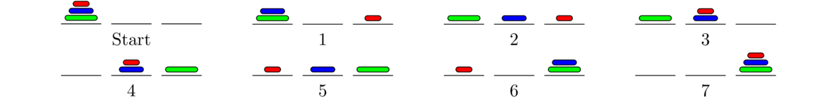
Looking carefully, we can see that the solution for two rings is used to solve the three-ring problem. Steps 1, 2, and 3 are the two-ring solution for moving two rings from the left to the center. Steps 5, 6, and 7 are the two-ring solution for moving two rings from the center to the right. And overall, the three-ring solution itself is structured like the two-ring solution. Now here's the solution for four rings:

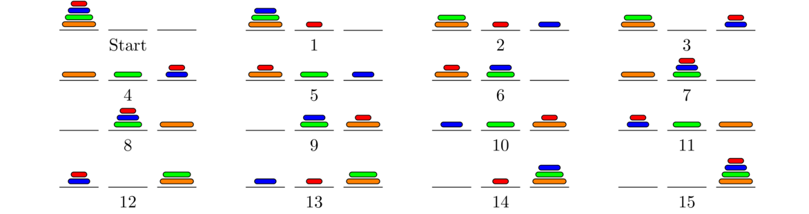
Notice that steps 1-7 use the three-ring solution to move the top three rings to the middle. Step 8 moves the big ring over the end, and then steps 9-15 use the three ring solution to move the top three rings over to the end.

Let's compare all of the solutions:

2 rings: Move the top ring to the center, move the bottom ring to the right, move the top ring to the right.
3 rings: Move the top two rings to the center, move the bottom ring to the right, move the top two rings to the right.
4 rings: Move the top three rings to the center, move the bottom ring to the right, move the top three rings to the right.

Shown below are parts of the two-, three-, and four-ring solutions, lined up, showing how they are similar.

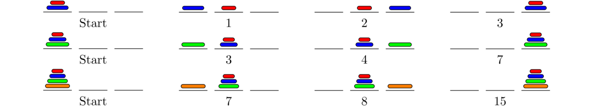
The general solution is a similar combination of the n-1 solution and the two-ring solution. We use the n-1 solution to move the top n-1 rings to the center, then move the bottom ring to the right, and finally use the n-1 solution to move the top three rings to the right.

It's not too hard to count the number of moves needed in general. The solution for two rings requires 3 moves. The solution for three rings requires two applications of the two-ring solution plus one more move, for a total of 2 · 3 + 1=7 moves. Similarly, the solution for four rings requires two applications of the three-ring solution plus one additional move, for 2 · 7+1=15 moves. In general, if h_n is the number of moves in the optimal solution with n rings, then we have h_n=2h_n-1+1. And in general, h_n=2ⁿ-1 moves.

This is exponential growth. Already, the solution for 10 pegs requires 2¹⁰-1=1023 moves. This is a lot, but doable by hand in under an hour. The solution for 20 pegs requires over a million moves, and the solution for 30 pegs requires over a billion moves. The solution for 100 pegs requires roughly 10³⁰ moves, which just might be able to be completed if every computer in existence worked round the clock for millions of years on the problem.

Here is a program that returns the optimal solution to the Towers of Hanoi problem:

import java.util.ArrayDeque;
import java.util.Deque;

public class Hanoi {
    private Deque<Integer> s1, s2, s3;

    public Hanoi(int n) {
        s1 = new ArrayDeque<Integer>();
        s2 = new ArrayDeque<Integer>();
        s3 = new ArrayDeque<Integer>();
        
        for (int i=n; i>=1; i--)
            s1.push(i);
        
        System.out.println(s1 + " " + s2 + " " + s3);
        recursiveHanoi(s1, s3, s2, n);
    }
    
    public void recursiveHanoi(Deque<Integer> start, Deque<Integer> end,
                               Deque<Integer> other, int size) {
        if (size==1) {
            end.push(start.pop());
            System.out.println(s1 + " " + s2 + " " + s3);    
        }
        else {
            recursiveHanoi(start, other, end, size-1);
            recursiveHanoi(start, end, other, 1);
            recursiveHanoi(other, end, start, size-1);        
        }
    }
    
    public static void main(String[] args) {
        new Hanoi(3);        
    }
}

Here is the output for the three-ring solution:

[1, 2, 3] [] []
[2, 3] [] [1]
[3] [2] [1]
[3] [1, 2] []
[] [1, 2] [3]
[1] [2] [3]
[1] [] [2, 3]
[] [] [1, 2, 3]

The code uses three stacks to represent the pegs. The class's constructor initializes the stacks and fills the left stack. All of the work is done by the recursiveHanoi method. The method takes three stacks—start, end, and other—as parameters, as well as an integer size. Any move can be thought of as moving size number of rings from start to end, using other as a helper peg.

The base case of the recursion is size=1, which is when we are moving a single ring from one peg to another. We accomplish that by popping the “peg” from the start stack and pushing it onto the end stack. At this point we also print out that stacks, so that every time a switch is made, the stacks are printed.

The recursive part of the method moves size-1 rings from the start stack to the helper stack (other), then moves the bottom ring from the start stack to the end stack, and finally moves size-1 rings from the helper stack to the end stack.

Working with recursion

In this section we look at a few nitty-gritty details of working with recursion.

Stack overflow errors

Here is the code from Section 4.1 that recursively reverses a string.

public static String reverse(String s) {
    if (s.equals(""))
        return "";

    return reverse(s.substring(1)) + s.charAt(0);
}

If we try running the reverse function on a really long string, we will get a stack overflow error. The reason for this is every time we make a recursive call, the program uses a certain amount of memory for local variables and other things the function needs. This is saved on an internal Java data structure called the call stack. This stack has a limited amount of space, typically space for maybe 10,000 function calls. Recursive calls are nested—each call happening before the previous one returns—which can cause the call stack to fill up, or overflow. This is a problem in most imperative languages, not just Java.

Here is another easy way to get a stack overflow error:

public static void f() {
    f();
}

Here we basically have an infinite recursive loop. This will eventually fill up the call stack and cause a stack overflow. When writing recursive code, it is easy for a program bug to cause a stack overflow. This often happens from making a mistake in the base case or forgetting it entirely. It can also happen if your recursive code does not actually break the input into smaller pieces. For instance, if instead of s.substring(1) in the reverse method, we use the entire string s itself, then the input string to the function will always be the same size, and the recursive calls will keep happening, never getting to the base case to stop the recursion. Eventually the call stack will overflow.

Using parameters

When working with recursion, it can be convenient to use function parameters as a kind of variable. For instance, consider the following ordinary code that counts to 10:

for (int i=1; i<=10; i++)
    System.out.print(i + " ");

Here is how to rewrite that code recursively:

public static void countToTen(int i) {
    System.out.print(i + " ");
    if (i == 10)
        return;
    else
        countToTen(i + 1);
}

Notice how the loop variable n from the iterative code becomes a parameter in the recursive code. In general, it's possible to convert any chunk of iterative code into recursive code using parameters in a similar way. As another example, here is some iterative code to compute Fibonacci numbers:

public static long fib(int n) {
    if (n==1 || n==2)
        return 1;
    
    long c=1, p=1;
    for (int i=0; i<n-2; i++) {
        long hold = c;
        c = p+c;
        p = hold;
    }
    return c;
}

Here is a direct translation of this approach into recursive code:

public static long fib(int n) {
    if (n==1 || n==2)
        return 1;
    return helperFib(n, 0, 1, 1);
}

private static long helperFib(int n, int i, long c, long p) {
    if (i==n-2)
        return c;
    return helperFib(n, i+1, c+p, c);
}

We have a helper function here because our recursive method has a lot of parameters that the caller shouldn't be bothered with. The fib function just handles the simple cases that n equals 1 or 2 and then sets the helperFib function in motion by essentially “initializing” the variable i to 0, and c and p to 1.

Notice how the variables in the recursive code (including the loop variable i) become parameters to the function. Also, notice how the for loop in the iterative code runs until i equals n-2, which is the base case of the helperFib function.

Let's compare the iterative code's for loop with the recursive call to helperFib.

for (int i=0; i<n-2; i++) {              return helperFib(n, i+1, c+p, c);
    long hold = c;
    c = p+c;
    p = hold;
}

Notice that the recursive function calls itself with the i parameter set to i+1, with the c parameter set to c+p, and with the p parameter set to c. This is the equivalent of what happens in the iterative code's for loop, where we do i++, c=c+p, and p=hold, where hold gets the old value of c.

This approach is more work than the earlier recursive Fibonacci method we wrote, but it runs much more efficiently than the other version. In general, a similar process to this can be used to translate any iterative code into recursive code. Note that it's actually the call stack that makes recursive solutions seem simpler than iterative ones. The call stack saves the value of the local variables, whereas with an iterative solution we have to keep track of the variables ourselves. In fact, we can convert a recursive solution into an iterative one by managing a stack ourselves.

The upshot of all this is that any (solvable) problem can be approached either iteratively or recursively.

Tail recursion

There is class of programming languages, called functional languages, which have better support for recursion than Java. They use what is called tail-call optimization to eliminate most of the overhead of the call stack. A function is said to be tail-recursive if it is written so that the last thing the function does is call itself without making any use of the result of that call other than to return it. Many of the examples from this chapter could easily be rewritten to be tail-recursive. For example, here is a tail-recursive version of the reverse method:

public static String reverse(String s) {
    return reverseHelper(s, "");
}

private static String reverseHelper(String s, String total) {
    if (s.equals(""))
        return total;
    return reverseHelper(s.substring(1), total + s.charAt(0));
}

Notice how the last thing we do is call the function, and nothing is done with the result of that other than to return it. This makes it tail recursive.

The reason for tail recursion is that some programming languages (but not Java as of this writing) can turn tail recursion into iterative code, eliminating the possibility for a stack overflow. Of course, why not just write the code iteratively to start? The answer is you should just write it iteratively, except that in some programming languages (mostly functional languages), you just don't (or can't) do that. In those languages, you write most things using recursion, and writing them in a tail-recursive way allows for the language's compiler to turn the code into iterative code that doesn't risk a stack overflow.

Summary

Sometimes recursion almost seems like magic. All you have to do is specify how to use the solution to the smaller problem to solve the larger one, take it on faith that the smaller one works, and you're essentially done (once you do the base case, which is often simple).

For example, here again is recursive solution to reversing a string: break off the first character, reverse the remaining characters and add the first character to the end. The code for this is:

return reverse(s.substring(1)) + s.charAt(0);

We just assume that reverse correctly reverses the smaller substring and then add the first character to the end. This, plus the base case to stop the recursion, are all that we need.

In Java, a simple rule for when to use recursion might be to use it when it gives a simpler, easier-to-code solution than an iterative approach and doesn't risk a stack overflow error or other inefficiency (like with the first Fibonacci function we did). A good example of an appropriate use of recursion is for calculating permutations. Iterative code to generate permutations is somewhat more complicated than the recursive code. And there is no risk of a stack overflow as we couldn't generate permutations for very large values of n recursively (or iteratively) because there are so many permutations (n! of them).

The take-home lesson is that in Java, most code is done iteratively, and recursion is useful on occasion.

Binary Trees

Introduction

Tree structures are fairly common. For example, shown below on the left is tree of the outcomes of flipping a coin three times. On the right is a simplified version of part of a phylogenetic tree showing the family relationships of animal species.

These are just two simple examples. Trees are especially important in computer science. Let's start with a little terminology. Consider the tree below.

The circles are called nodes. Each node has a data value associated to it. The node at the top of the tree is called the root. Each node may or may not have some child nodes. The nodes at the end of the tree (that have no children) are called leaves. Of particular interest are binary trees, trees where each node can have up to two children, but no more.

Implementing a binary tree

Let's look at how we can build a binary tree class. One approach is to use nodes, similar to what we did with linked lists. The main difference from linked lists will be that our Node class will have two links, one pointing to the left child and one pointing to the right child. Also, we will use root to refer to the first node, as opposed to front for linked lists. Here is the framework of the class:

public class BinaryTree<T> {
    private class Node {
        public T value;
        public Node left
        public Node right;
    
        public Node(T value, Node left, Node right) {
            this.value = value;
            this.left = left;
            this.right = right;
        }
    }
        
    private Node root;
    
    public BinaryTree()    {
        root = null;
    }
}

Notice the similarity to the linked list class. Next, we will consider how to add a new node to the tree. We will allow callers to add to any location in the tree. To do this, callers will specify a string of L's and R's, indicating how to traverse the tree by moving left and right to get to where the new node should go. For instance, the figure below shows the addition of a node with data value 8 as the left child of the node with data value 1.

To get to the place to add the new node, starting at the root we would have to walk left and then right, and then add the new node as the left child. The caller could do this via add(8, "LRL"). The first two letters, "LR", tell how to get to the insertion point, and the last letter, L, says to insert the new node as the left child. Here is code that implements this addition process:

public void add(T value, String location) {
    if (location.equals("")) {
        root = new Node(value, null, null);
        return;
    }
    
    Node node = root;
    for (char c : location.substring(0, location.length()-1).toCharArray()) {
        if (c == 'L')
            node = node.left;
        else
            node = node.right;
    }
    
    if (location.charAt(location.length()-1) == 'L')
        node.left = new Node(value, null, null);
    else
        node.right = new Node(value, null, null);
}

The first case, where the location is an empty string, is how the user would add something to the root of the tree. Otherwise, we use all the characters of the location string except the last to move us to the right spot in the tree. Once we get there, we use the last character to tell us whether to add the new node as the left or right child.

Note that if the caller specifies a location that is already in the tree, then this code will wipe out a portion of the tree.

Binary trees and recursion

Most of the methods we will write for binary trees will be recursive. This is because a binary tree is itself recursive. The left child of a node and all of its descendants form a tree (a subtree), as do the right child and its descendants.

A size method

The first method we write tells how many nodes are in the tree. Before we write it, let's look at a recursive method that returns the length of a string:

public static int length(String s) {
    if (s.equals(""))
        return 0;
    return length(s.substring(1)) + 1;
}

We break the string into its head (the current character) and tail (everything after it), and the overall length is the length of the tail plus 1 for the head. Here now is the binary tree size method:

public int size(Node node) {
    if (node == null)
        return 0;
    return size(node.left) + size(node.right) + 1;
}

Whereas we break strings up into their head and tail, for binary trees it's more like there are two tails: a left and a right one. The size of the tree that starts at a given node is the size of the left subtree plus the size of the right subtree, plus 1 for the node itself. See the figure below.

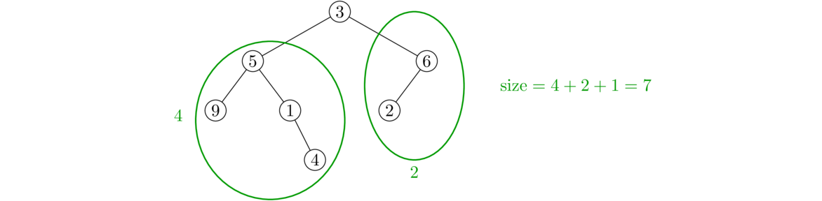
Note the base case is a null node. The ends of the tree are indicated by nulls, so that is where we stop the recursion.

One issue with this approach is that the recursion requires a Node parameter, but someone calling the method just wants to do something like tree.size() without having to worry about a Node parameter. To fix this, we introduce a helper, as below:

public int size() {
    return sizeHelper(root);
}

private int sizeHelper(Node node) {
    if (node == null)
        return 0;
    return sizeHelper(node.left) + sizeHelper(node.right) + 1;
}

The helper method does all the work. The size method is a wrapper around it that simply starts the recursion in motion at the tree's root.

We will look at several other binary tree methods. Each will follow the same structure as this one. The way to approach these problems is to ask the following: if we know the answer to the problem for the left and right subtrees, how can we combine that along with information about the node itself to answer the overall problem?

A contains method

Here we look at a method that tells whether or not the tree contains a particular data value. To write it recursively, we use the same approach as with the size method. We look at the current node itself, its left subtree, and its right subtree. In particular, the subtree starting at a particular node contains a given data value if that data value is either at the node itself, in its left subtree, or in its right subtree. See the figure below:

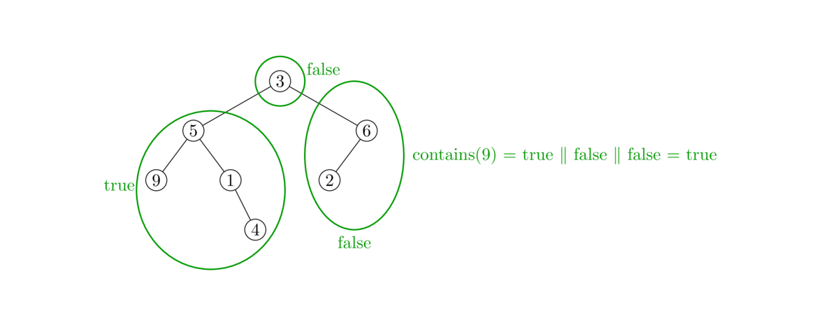
Here is how we code the method:

public boolean contains(T value) {
    return containsHelper(value, root);
}

private boolean containsHelper(T value, Node node) {
    if (node == null)
        return false;
    
    return node.value.equals(value) || containsHelper(value, node.left) ||
           containsHelper(value, node.right);
}

Just like with the size method, we use a helper method. The base case is a null node. The recursive part checks the node itself for the data value and it recursively checks the left and right subtrees. We use a single statement here to return the logical OR of the three possibilities, but we could also do this with an if/else statement.

A height method

The height of a tree is how many levels deep it goes. An empty tree's height is 0. A tree with just a root has height 1. A tree that has a root with one or two children and no other nodes has height 2. In general, an element is said to be at level k of the tree if we have to follow k links to get to it from the root. The root is at level 0, the root's two children are at level 1, their children are at level 2, etc. The tree's height is how many levels it has.

Knowing the heights of the left and right subtrees, how do we get the overall height? Take whichever of the two heights is larger and add 1 to it since the current node adds 1 to the total height. See the figure below:

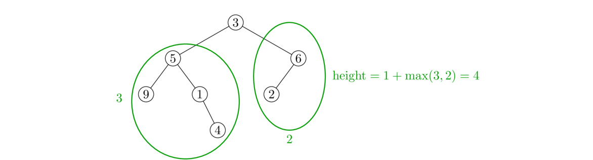
Below is the code for the method. Note that Java's Math.max method returns the larger of two numbers.

public int height() {
    return heightHelper(root);
}

private int heightHelper(Node node) {
    if (node == null)
        return 0;
    
    return 1 + Math.max(heightHelper(node.left), heightHelper(node.right));
}

This height method demonstrates how to think recursively: figure out how the problem can be solved in terms of smaller versions of itself. You don't actually have to specify how to move through the tree. Instead specify how to combine the solutions to the subproblems to get a solution to the whole, and specify a base case to stop the recursion.

A method to count leaves

The leaves of a tree are the nodes at the ends of the tree that don't have any children. In terms of Java code, a node called node is a leaf if node.left and node.right are both null. We can combine this fact along with recursion to count the number of leaves in a tree. In particular, the number of leaves is the number of leaves to the left of the current node plus the number to the right. See the figure below:

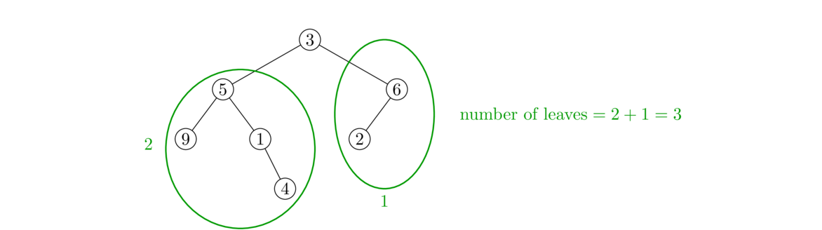
Here is the code:

public int countLeaves() {
    return countLeavesHelper(root);
}

public int countLeavesHelper(Node node) {
    if (node == null)
        return 0;
    if (node.left == null && node.right == null)
        return 1;
    return countLeavesHelper(node.left) + countLeavesHelper(node.right);
}

There are essentially two base cases here, one for when we fall off the end of the tree and one for if the node is a leaf.

A toString method

Here we write a toString method for printing all the elements in the tree. The method follows the same basic structure as all of the other methods we have written. Here is the code:

@Override
public String toString() {
    return toStringHelper(root);
}

private String toStringHelper(Node node) {
    if (node == null)
        return "";
    else
        return toStringHelper(node.left) + node.value + " " + toStringHelper(node.right);
}

This code walks recursively through the tree in a particular order called an in-order traversal.

The way that works is we always visit nodes in the order left-center-right. That is, from any given node, we will always print out everything in the left subtree, then the node's own value, and finally everything in its right subtree. This is a recursive process. From a given node we first print out the in-order traversal of the left subtree, then the value of the node, then the in-order traversal of the right subtree. Let's look at how this works on the tree below:

Start at the root. According the in-order rule, we first look at its left subtree. So we're now at the node labeled with 5. Again, recursively following the rule, we look at this node's left subtree. We're now at the node labeled 9. Its left subtree is empty, so following the in-order rule, we then look at the node itself, which has data value 9, and that's the first thing that gets printed. The node labeled 9 has no right subtree. Having finished with this node, we back up to the previous node. Having finished its left subtree, we visit the node itself, and print out a 5. We then visit its right subtree and apply the same process. In the end, we get 9 5 1 4 3 6 2.

If we change around the order in the return statement we can get other types of traversals. Two common ones are the pre-order traversal (node, left, right) and post-order traversal (left, right, node).

Below is an alternate toStringHelper method that prints out the path to each node as a string of L's and R's. To get the path, we add a parameter location to the helper function. In the recursion, we add an "L" or "R" to the previous value of location depending on whether we are moving on to the left or right subtree. This location variable thus keeps track of the string of L's and R's that we have to take from the root to get to the node.

private String toStringHelper(Node n, String location) {
    if (n == null)
        return "";
    
    if (n == root)
        return toStringHelper(n.left, location+"L") + " " + "root: " + n.value +
               "\n" + toStringHelper(n.right, location+"R");
    
    return toStringHelper(n.left, location+"L") + " " + location + ": " +
           n.value + "\n" + toStringHelper(n.right, location+"R");
}

For the tree shown earlier in this section, here is the output of this method:

LL: 9
L: 5
LR: 1
LRR: 4
root: 3
RL: 2
R: 6

Returning the things at even levels

Here is one more example, this one a little trickier. Suppose we want to return a string containing only the data that is at even levels (levels 0, 2, 4, etc.), namely the root, it's grandchildren, great-great grandchildren, etc. We need some way of keeping track of what level we are at. We can do that by adding a parameter called level to the recursion. Each time we make a recursive call, we use level+1, which has the effect of remembering what level each node is at. The rest of the code is similar to the toString method. Here it is:

public String stuffAtEvenLevels() {
    return stuffAtEvenLevelsHelper(root, 0);
}

public String stuffAtEvenLevelsHelper(Node node, int level) {
    if (node == null)
        return "";
    if (level % 2 == 0)
        return stuffAtEvenLevelsHelper(node.left, level+1) + node.value + " " +
               stuffAtEvenLevelsHelper(node.right, level+1);
    else
        return stuffAtEvenLevelsHelper(node.left, level+1) +
               stuffAtEvenLevelsHelper(node.right, level+1);
}

More about binary trees

Running times of the methods

All of the recursive methods we wrote have to visit all of the nodes in the tree. They all run in O(n) time.

The add method is a little different. It runs in O(n) in the worst case. The worst case here is if the tree is a path, where all the nodes are strung out essentially in a line, with each node except the last having exactly one child. If we try to add to the bottom of a tree of this form, we have to walk through all n nodes to get to the bottom of the tree. On the other hand, if the tree is more-or-less balanced, where for any given node both its left and right subtrees have roughly the same size, then adding is O(log n). This is because with each left or right turn we take to get to the desired node, we essentially are removing half of the tree from consideration. These ideas will be especially important in the next chapter.

A different approach

There is another approach we can take to implementing binary trees that is simpler to code, but less user-friendly to work with. The key observation here is to think of a tree as a recursive data structure. Each node of the tree consists of a data value and links to a left and a right subtree. And those subtrees are of course binary trees themselves. Here is how such a class might look (using integer data for simplicity):

public class Tree {
    private int value;
    private Tree left, right;
    
    public Tree(int value, Tree left, Tree right) {
        this.value = value;
        this.left = left;
        this.right = right;
    }
}

Here a binary tree and its declaration using this class. The declaration is spread across several lines for readability.

Tree tree = new Tree(3,
                     new Tree(5,
                              new Tree(9, null, null),
                              new Tree(1, null, null)),
                     new Tree(6, null, null));

We could then add methods to our class if we want. Here's a toString method:

@Override
public String toString() {
    return toStringHelper(this);
}

public String toStringHelper(Tree tree) {
    if (tree==null)
        return "";
    return toStringHelper(tree.left) + " " + tree.value + toStringHelper(tree.right);
}

We can see that this is very similar to the earlier toString method. In fact, the other recursive algorithms we wrote would change very little with this new approach.

This approach and the earlier node-based approach are actually quite similar. In the earlier approach the recursion is hidden in the Node class, which has references to itself.

Either of the two implementations of binary trees gives a good basis to work from if you need a binary tree class for something. This is important as there is no binary tree or general tree class in Java's Collections Framework, so if you need an explicit binary tree class, you either have to code one up yourself or look around for one.

Applications

Binary trees and more general trees are a fundamental building block of other data structures and algorithms and form a useful way to represent data. They show up in networking algorithms, compression algorithms, and databases. In Chapters 6 and 7 we will see binary search trees and heaps, which are specialized binary trees used for maintaining data in order.

A computer's file system can be thought of as a tree with the directories and files being the nodes. The files are leaf nodes, and the directory nodes are nodes whose children are subdirectories and files in the directory.

Another place binary trees show up is in parsing expressions. An expression is broken down into its component parts and is represented using a tree like in the example below, which represents the expression 3+4*5-6.

Trees also provide a natural way to structure moves from a game. For example, the potential moves in a game of tic-tac-toe can be represented with a tree as follows: The root node has nine children corresponding to nine possible opening moves. Each of those nodes has eight children corresponding to the eight possible places the second player can go. Each of those nodes has children representing the first player's next move. And those children have children, and so on to the end of the tree. A computer player can be implemented by simply searching through the tree looking for moves that are good according to some criterion.

Binary trees are also one of the simplest examples of graphs, covered in Chapter 10.

Binary Search Trees

Introduction

Suppose we have some data that is in order. We are continually adding and deleting things, and we want the data to stay in order as things are added and deleted. One approach is to store the data in a list and use a search to find the right place to add new elements, or just add new elements to the end of the list and re-sort it. This is fine if the list is small or if we don't care about speed. However, list insertions, as well as deletions, are typically O(n), and a list sort is an O(n log n) operation typically.

By storing our data in a more clever way in something called a binary search tree (BST), we can get the running time down to O(log n). It is worth noting once more how big a difference there is between n and log n: if n=1,000,000}, then log n = 20. There is a huge difference between a program that takes 1,000,000 microseconds to run and a program that takes 20 microseconds to run.

Recall from Section 1.5 that the binary search algorithm is an O(log n) algorithm for finding an element in a list. It works by breaking continually breaking the data into halves and only looking at the halves that could contain the value we are looking for. We start by looking at an entry in the middle of the list. Assuming we don't find it on the first try, if the entry is bigger than the one we want we know not to bother with the upper half of the list and to just look at the lower half of the list, and if the entry is smaller than the one we want, we can just focus on the upper half of the list. We then apply the same procedure to the appropriate half of the list and keep doing so, cutting the search space in half at each step until we find the value we want. This continuous cutting in half is characteristic of logarithmic algorithms.

A BST can be thought of as combination of a binary tree and the binary search algorithm. Formally, a BST is a binary tree with one special property:

For any given node N, each element in its left subtree is less than or equal to the value stored in N and each element in its right subtree is greater than the value stored in N.

Below are two binary trees. The one on the left is a binary search tree, but the one on the right is not. Notice in the tree on the left that for any given node, everything to the left of it is less than or equal to it and everything to the right is greater than it. On the other hand, the tree on the right is not a binary search tree for two reasons. First, the 16 in the third level is greater than the 14 at the root but is to the left of 14. Second, the 17 at the bottom of the tree is less than 18 two levels up from it but is to the right of it.

Adding and deleting things

Adding things

To add an element to a BST we rely on the key property of BSTs, that things to the left of a node are smaller and things to the right are larger. We start at the root and traverse the tree comparing the value to be added to the value stored in the current node. If the value to be added is less than or equal to the value in the current node, we move left; otherwise, we move right. We continue this until we reach the end of the tree (reach a null link).

For instance, in the example below, let's suppose we are adding a 7 into the BST.

We start by comparing 7 to the root's value 5. Since 7>5, we move right. Then we compare 7 to the next node's value, 11, and since 7≤ 11, we move left. Then comparing 7 to 6, we see 7>6 so we move right. At this point we stop and add the new node because the last move right led to a null node at the end of the tree.

Here is another example. Suppose we add the integers 5, 11, 19, 6, 2, 4, 2, 3, 26 to the BST in exactly that order. The figure below shows the evolution of the tree.

Try this on paper for yourself to get a good sense of how the BST property works.

It might not be obvious that the data stored in this tree is actually sorted, but it is. The key is to do an in-order traversal of the tree. Remember that an in-order traversal visits nodes in the order left-middle-right, visiting the entire left subtree, then the node itself, then the right subtree. The BST property guarantees that the data values of everything to the left of a node will be less than or equal its value and everything to the right will be greater, which means that an in-order traversal will return the data in exactly sorted order.

Deleting things

When deleting things from a BST, we sometimes have to be careful. There are three cases to consider: (1) deleting a leaf, (2) deleting a node with exactly one child, (3) deleting a node with two children.

Deleting a leaf

Deleting a leaf is pretty straightforward. We simply remove the leaf from the tree. Doing so has no effect on the BST property. See below.

Deleting a node with exactly one child

Here we have to be a little more careful. We can't just remove the node from the tree, as that would create a hole in the tree. Instead, we reroute the link from the deleted node's parent to point to that node's (only) child. See below.

Deleting a node with two children

This is the most interesting case. We can't reroute the parent's link to the child like in the previous case because there are two children. Rather, the trick is to replace the node being deleted with the largest node in left subtree of the node being deleted. See the figure below for an example.

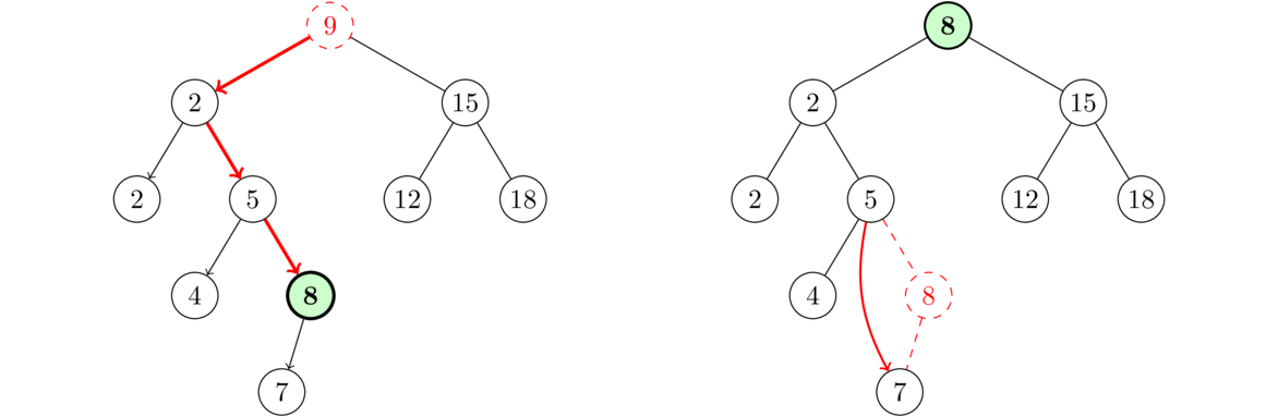
Why does this work? Let d be the name of the node being deleted and let m be the largest node in the left subtree of d. Because m is to the left of d, it is guaranteed to be less than anything to the right of d, so that part of the BST property works. Further, since m is the largest thing in the left subtree, it is guaranteed to be greater than everything to the left of d, so that part of the BST property is satisfied. So, overall, m fits perfectly into the tree right where d is.

One other potential problem is about how to delete m since we are moving it from its current location. The fact is that m is guaranteed to have no right child since any such child would have to be larger than m, and m is the largest thing in that subtree. So m has at most one child, so we can just delete it if it's a leaf or reroute its parent's link around it if it has a left child.

It's worth asking if this is the only way to do things. The answer is no. By symmetry, we could replace the deleted node with the smallest thing in its right subtree. There are often other things that we could replace it with, but in order to program this, we want to have some rule that always works, and this rule is guaranteed to work. It's also fast, running usually in O(log n) time (we'll see why a little later).

Running times

An important consideration about BSTs is how well balanced they are. Roughly speaking, a tree is balanced if all of the paths from the root to the leaves (nodes at the ends of the tree) are roughly the same length. If there are some long and some short paths, the tree is unbalanced. The tree on the left below is balanced, while the one on the right is not.

In the perfectly balanced case, each of the paths from the root to the leaves has length log n, where n is the number of nodes. To see why, note that at the root level there is one node. At the next level there are at most two nodes, the root's two children. At the next level, each child has at most two children for a total of four nodes. In general, as we go from level to the next, the maximum number of nodes doubles, so we have 2^k-1 nodes at level k, where level 1 is the root level. If the tree is completely full to level k, then, using the geometric series formula, we find that there are 1+2+4+…+2^k-1 = 2^k-1 total nodes in the tree. Thus we see that a tree with n nodes and k levels must satisfy the equation 2^k-1=n. Solving for k, we get k=log(n+1). So the number of levels is the logarithm of the number of nodes. Another way to look at things is that each time we choose a left or right child and step down the tree, we cutting off half of the tree. This continual dividing in half is just like the binary search algorithm, which has a logarithmic running time. In a case like this, adding and checking if the tree contains an item will both work in O(log n) time as they both walk down the tree one level at a time, until they reach their goal or the bottom of the tree. Deleting an item will also work in O(log n) time, as it won't take more than O(log n) steps to find the largest item in the left subtree.

As long as the tree is relatively balanced, the methods will work in more or less O(log n) time. If there is a lot of data and it's pretty random, the tree will be fairly well balanced. On the other hand, suppose the data we're putting into a BST already happens to be sorted. Then each item as its added to the BST will be added as the right child of its parent. The result is a degenerate tree, a long string of nodes, arranged like in a list. In this case the BST behaves a lot like a linked list and all the operations are reduced to O(n). This is a serious problem because in a lot of real life situations, data is often sorted or nearly sorted.

In a case like this, there are techniques to balance the tree. One of these techniques, AVL trees, involves rebalancing the tree after each addition of a node. This involves moving around a few nodes in the area of the added node. Another technique is red-black trees. These techniques are nice to know, but we will not cover them here. They are covered in other data structures books and on the web.

Java's Collections Framework does not have a dedicated BST class, though it does use BSTs to implement some other data structures (like sets and maps, which we'll see in Chapter 8).

Implementing a BST

A binary search tree is a binary tree, so we can use the same binary tree class we already wrote as a base. Here is the start of the class along with a toString method:

public class BinarySearchTree {
    private class Node {
        public int value;
        public Node left;
        public Node right;
        public Node(int value, Node left, Node right) {
            this.value = value;
            this.left = left;
            this.right = right;
        }
    }

    private Node root;

    public BinarySearchTree() {
        root = null;
    }

    @Override
    public String toString() {
        return toStringHelper(root);
    }

    public String toStringHelper(Node node) {
        if (node == null)
            return "";
        else
            return toStringHelper(node.left) + node.value + " "
            + toStringHelper(node.right);
    }

The toString method works in the order left-center-right. Keeping in mind the BST property about everything left being less and everything right being greater, this toString method will always print out the BST's data in perfectly sorted order.

Adding things to a BST

The process for adding a value to a BST is as follows: Start at the root, compare the value to it, move left if it's less than or equal to the root's value and move right otherwise. At the next node, we repeat the process. We continue until we reach the end of the tree (a null node) and then insert a new node at that location. This is all coded below:

public void add(int value) {
    if (root == null) {
        root = new Node(value, null, null);
        return;
    }

    Node node = root;
    Node parent = null;
    while (node != null) {
        parent = node;
        if (value <= node.value)
            node = node.left;
        else
            node = node.right;
    }
    if (value <= parent.value)
        parent.left = new Node(value, null, null);
    else
        parent.right = new Node(value, null, null);
}

At the start of the code we have a special case for adding to an empty tree. After that we have the code that walks the tree, moving left or right depending on how the inserted value compares to the current node's value.

Once we are done with that, we create the new node and insert it as either the left or the right child of the last tree node we reached. In order to keep track of that last tree node, we use a separate Node variable called parent. In the loop, before we update the variable node, we set parent=node. The effect is that as we walk through the tree, node is the current node we are at and parent is the one we were at in the previous step.

Here is some code to test the add method:

BinarySearchTree bst = new BinarySearchTree();
List<Integer> list = new ArrayList<Integer>();
Collections.addall(list, 5, 11, 19, 6, 2, 4, 2, 3, 26);
for (int x : list)
    bst.add(x);
System.out.println(bst);

And the output looks like below, in perfectly sorted order:

2 2 3 4 5 6 11 19 26

Checking if the tree contains a given value

The code for checking for containment is very similar to the code for the add method. We have a very similar loop that walks through the tree, moving left or right as appropriate. If in the loop we ever find the value we are looking for, we return true. If we fall off the end of the tree, then we are guaranteed by the BST properties that the value is not in the tree, so we return false.

public boolean contains(int value) {    
    Node node = root;
    while (node != null) {
        if (node.value == value)
            return true;
        else if (value < node.value)
            node = node.left;
        else
            node = node.right;
    }
    return false;
}

Deleting things

Recall that there are three cases to deleting a node: (1) deleting a leaf (a node with no children), (2) deleting a node with exactly one child, and (3) deleting a node with exactly two children. This method is arguably the most complicated one in this book. First, here is the entire method:

public void delete(int value) {
    // Special case if removing root and root doesn't have 2 children
    if (root.value == value && root.left == null) {
        root = root.right;
        return;
    }
    if (root.value == value && root.right == null) {
        root = root.left;
        return;
    }

    // Get to the node being deleted
    Node node = root;
    Node parent = null;
    while (node.value != value) {
        parent = node;
        if (value < node.value)
            node = node.left;
        else
            node = node.right;
    }

    // Case 1: Deleting a leaf
    if (node.right == null && node.left == null) {
        if (node == parent.left)
            parent.left = null;
        else
            parent.right = null;
    }

    // Case 2a: Deleting a node with only a left child
    else if (node.right == null) {
        if (node == parent.left)
            parent.left = node.left;
        else
            parent.right = node.left;
    }

    // Case 2b: Deleting a node with only a right child
    else if (node.left == null) {
        if (node == parent.left)
            parent.left = node.right;
        else
            parent.right = node.right;
    }

    // Case 3: Deleting a node with 2 children
    else {
        Node largest = node.left;
        Node parentOfLargest = node;

        while (largest.right != null) {
            parentOfLargest = largest;
            largest = largest.right;
        }
        node.value = largest.value;
        if (parentOfLargest == node)
            parentOfLargest.left = largest.left;
        else
            parentOfLargest.right = largest.left;
    }
}

The code starts off with a special case involving the root that isn't covered by any of the later cases. After that, we have a loop, very similar to the loop in the add and method, that locates the node to be deleted as well as its parent.

We then take care of deleting a leaf. To do that, we break the link from its parent, using an if statement to figure out if the node is its parent's left or right child.

The next part of the code handles deleting a node with one child by routing the link from the parent around the child to point to the grandchild.

The last part of the code handles deleting a node with two children. Recall that to do that, we replace the deleted node with the largest value in its left subtree. To find that node, we move left from the deleted node and then move right as far as we can until we hit the end of the tree. The node we reach in that way is guaranteed to be the largest in the left subtree.

We then replace the deleted node's value with the value we just found and we delete the node we just found by routing its parent's link around it to its left child (which might be null). There won't be a right child since we found that node by going right as far as we could. Note that we need a special case to handle to possibility that the largest thing in the left subtree is actually the left child of the node being deleted.

It's good to stress-test this method a bit. Below is some code to do that. The code adds 100 random integers to a BST and then randomly chooses elements to delete from the tree.

List<Integer> list = new ArrayList<Integer>();
Random random = new Random();

for (int i=0; i<100; i++)
    list.add(random.nextInt(100) + 1);

BinarySearchTree bst = new BinarySearchTree();
for (int x : list)
    bst.add(x);
System.out.println(bst);

Collections.shuffle(list);
for (int x : list) {
    bst.delete(x);
    System.out.println(bst);
}

When we run the code, at each stage we should see the tree shrink by 1 item, and there should be no errors (especially no null pointer exceptions).

A generic BST

The BST above only works with integer data. In this section we will talk about how to get it to work with generics. We can't just add a <T> to the declaration and change int to T elsewhere. The reason is that we have to be able to compare the data values to each other. We can compare numbers by value and we can compare strings alphabetically, but some data types don't have a natural way of being compared. For instance, suppose we have a data type representing colors. How would we say if red is less than green or if brown is greater than gray? Or if we had a data type representing fruits, we would literally have to compare apples and oranges.

Java's `Comparable` interface

In Java, the way to signify that something is able to be compared is for it to implement the Comparable interface. Anything that implements this interface is guaranteed to have a compareTo method that tells how to compare two elements of that type. The rules of the compareTo method are that if we have objects a and b and we call a.compareTo(b), the method should return a negative integer if a is less than b, 0 if a and b are equal, and a positive integer if a is greater than b.

Java's built-in Integer, Double, and String classes all implement the Comparable interface. For instance, the following prints out a negative number:

System.out.println("abc".compareTo("def");

Here is an example of how to create a class that implements the Comparable interface. Say we have a class representing a playing card. The card has a suit and a value, and we want to compare cards based on their values. Here is how to do that:

public class Card implements Comparable<Card> {
    private int value;
    private String suit;

    public Card(int value, String suit) {
        this.value = value;
        this.suit = suit;
    }

    public int compareTo(Card other) {
        return ((Integer)this.value).compareTo(other.value);
    }    
}

The compareTo method for this class piggybacks off the compareTo method of Java's built-in Integer class. Here is how we would use the class to compare cards:

Card a = new Card(3, "diamonds");
Card b = new Card(10, "hearts");
if (a.compareTo(b) < 0)
    System.out.println("a is the smaller card");
else
    System.out.println("b is the smaller card");

Making the BST class work with comparable objects

To rewrite the binary search tree class using generics, we have only a few changes to make. First, here is the declaration of the class:

public class BinarySearchTreeGeneric<T extends Comparable<T>>

The exact syntax is important here. It basically says that our BST class will be able to work with any data type for which a way to compare objects of that type has been defined. Specifically, anything that implements Comparable must have a compareTo method, and that is what our BST class will use. We then go through and replace all occurrences of int data with T data. We also replace comparisons using <, <=, etc. with their equivalent compareTo form as shown in the table below.

Ordinary	`compareTo`
`a < b`	`a.compareTo(b) < 0`
`a <= b`	`a.compareTo(b) <= 0`
`a == b`	`a.compareTo(b) == 0`
`a != b`	`a.compareTo(b) != 0`
`a > b`	`a.compareTo(b) > 0`
`a >= b`	`a.compareTo(b) >= 0`

For example, here is how the contains method changes:

public boolean contains(int value) {        public boolean contains(T value) {        
    Node node = root;                           Node node = root;
    while (node != null) {                      while (node != null) {
        if (node.value == value)                    if (node.value.compareTo(value) == 0)
            return true;                                return true;
        else if (value < node.value)                else if (value.compareTo(node.value) < 0)
            node = node.left;                           node = node.left;
        else                                        else
            node = node.right;                          node = node.right;
    }                                           }
    return false;                               return false;
}                                           }

Heaps

Introduction

A heap is another kind of binary tree. Like BSTs, heaps maintain their elements in a kind of sorted order. The main property of heaps is that they are a way to store data in which continually finding and possibly removing the smallest element is designed to be very fast. In particular, finding the minimum element in a heap is a O(1) operation, compared with O(log n) for a BST. However, unlike BSTs, heaps do not store all the data in sorted order. It's just the minimum value that is guaranteed to be easy to find.

The definition of a heap is that it is a binary tree with two special properties:

The value of a parent node is less than or equal to the values of both its children.
The nodes are added into the tree typewriter style. That is, we start at the root and move through the tree from left to right, completely filling a level before moving on to the next. The order is shown in the figure below.

Notice the difference in property 1 between BSTs and heaps. In a BST, values to the left of the parent are always less than or equal to the parent's value and values to the right are larger. In a heap, left and right are not important. All that matters is that the values of the parent be less than or equal to the values of its children. Property 2 guarantees that the heap is a balanced binary tree.

The heap described above is a min-heap. We can also have a max-heap, where the “less than” in property 1 is changed to “greater than.”

Below on the left is a binary tree that is a heap, and on the right is a binary tree that is not a heap. Notice in the left tree that every parent is less than or equal to its child. Remember also that this is not a BST, so it's okay if the left child is larger. Notice further that the tree has no gaps. An entire level is filled up before moving on to the next level.

On the other hand, the tree on the right is not a heap for two reasons. First, the node with value 12 has a child with value 9, breaking the rule that the parent has to be less than or equal to the child. Second, there is a hole where the node with value 4 should have a left child. This tree was not filled typewriter-style.

Adding and removing things

Adding to a heap

When we add an item to a heap, we have to make sure it is inserted in a spot that maintains the heap's two properties. To do this, we first insert it at the end of the heap. This takes care of the second property (completely filling the heap left to right, typewriter style), but not necessarily the first property (parent's data less than or equal to its children's data). To take care of that, we compare the inserted value with its parent. If it is less than its parent, then we swap child and parent. We then compare the inserted value to the parent's parent and swap if necessary. We keep moving upward going until the first property is satisfied or until we get to the root. The new item sort of bubbles up until it gets to a suitable place in the heap.

Below is an example where we add the value 3 (shown in green) to the heap. We start by placing it at the end of the heap. Its value is out of place, however. We compare its value to its parent, which has value 8. Since 3<8, a swap is necessary. We then compare 3 with its new parent, which has value 5. Since 3<5, another swap is needed. We again compare 3 with its new parent and this time 3>1, so we can stop.

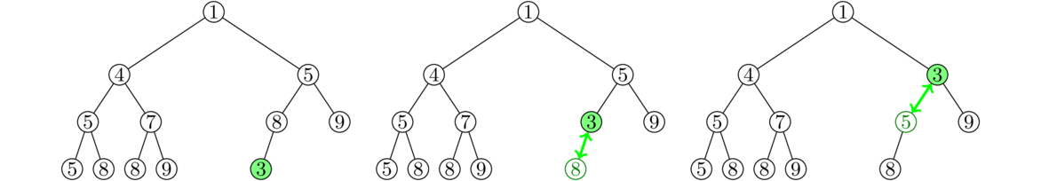
Popping from a heap

Popping from a heap is a little tricky because we have to move things around to fill in the gap left by removing the top. The idea here is similar to what we did with adding an element, just done in reverse. What we do is take the last element, x, in the heap and move it to the top. This ensures that property 2 is satisfied. But doing so will probably break property 1, so we compare x with its children and swap if necessary with the smaller child. We then compare x with its new children and swap again if necessary. We continue this until property 1 is satisfied. Essentially, the item sinks until it reaches a suitable place in the heap. When doing the comparisons, we always swap with the smaller of the two children to ensure that property 1 holds. Below is an example:

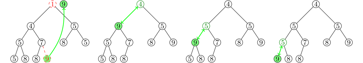
In the example we start by moving the very last item (value 9) from the end of the heap to the top. Specifically, that value of 9 is deleted from the bottom and it replaces the value at the top of the tree. We then compare 9 to its two new children, 4 and 5. Since 9 is out of place, being larger than them, we swap it with the smaller child, 4. We then repeat the process with 9's two new children, and then repeat the process one more time until 9 ends up at the right place in the heap.

Running time and applications of heaps

Running time of the methods

The peek method, which returns (but does not remove) the minimum value of a heap, is O(1). This is because the minimum value is always stored at the top of the heap and it is a quick operation to look at that value and return it.

The add and pop methods of heaps each run in O(log n) time. In the worst case scenario, each method will require a number of swaps equal to the number of levels in the tree. The heap is a complete binary tree, so the number of levels is the logarithm of the number of nodes in the tree.

Since the add method runs in O(log n) time, building a heap from a list n elements will run in O(n log n) time.^**There does exist an O(n) algorithm for doing that, but it is beyond the scope of this book.

Applications of heaps

Repeatedly popping elements off of a heap returns the values in order from least to greatest. So heaps can be used to sort data. This sort is called heapsort and it is one of the faster sorts out there. We will have more to say about it in Chapter 11. Heaps are also used to implement certain important graph algorithms for things like finding spanning trees and shortest paths. In general, heaps are useful when you are continually adding things to a data structure and need quick access to the smallest or largest value added.

Here's a longer example: An important type of simulation is simulating a large number of particles that can collide with one another. This shows up in computer games and in simulations of molecules, among other places. Let's say we have n particles. Usually simulations work by setting a small time step, say .001 seconds, and at every time step we advance all the particles forward by the appropriate amount. At each time step we then have to check for collisions. One way to go about checking for collisions is to loop through the particles and for each particle, loop through the other particles, checking to see which are about to collide with the current particle. This requires a total of n(n-1)/2 checks, which is a lot of checks to be making every .001 seconds.

We can greatly reduce the number of checks using a heap. First assume that the particles are moving in straight line trajectories. We can calculate ahead of time when two particles will collide. We use a heap of collisions, with the heap values being the collision times. After each time step we pop off any imminent collisions from the heap and address them. It may happen that a collision we calculated ahead of time may not happen because one of the particles got deflected in the meantime, so we also keep track of which collisions won't happen. After addressing collisions, we have to recalculate new collisions since the colliding particles are now moving in different directions, but the total number of these calculations is usually a lot less than n(n-1)/2.

Heaps in the Collections Framework

Java doesn't have a class specifically called a heap, but it does have something called a priority queue, which can be used as a heap. A priority queue is a queue where each element is given a priority and when elements are removed from the queue, they are removed in order of priority. Lots of real-life situations can be described by priority queues. For instance, in our everyday lives we have a bunch of things to do, some of which have higher priorities than others. In computers, operating systems use priority queues to determine which tasks to run when, as certain tasks are more important than others.

Internally, Java's PriorityQueue class is implemented with a heap, and we can use the PriorityQueue as a heap. Here is an example:

PriorityQueue<Integer> heap = new PriorityQueue<Integer>();

heap.add(8);
heap.add(4);
heap.add(1);
heap.add(2);

for (int i=0; i<4; i++)
    System.out.print(heap.remove() + " ");

The remove method will pop things off in numerical order, and the output will be 1 2 4 8. Note further that the method that returns the top value without removing it is called element.

Implementing a heap

Shown below is a heap with the nodes labeled in order by level, left to right. Remember that a heap has no gaps. So this suggests that we can represent a heap using a list, specifically a dynamic array. In particular, the root will be at list index 0, its two children will be at indices 1 and 2, its left child's children will be at indices 3 and 4, etc.

Shown below is an example heap and its dynamic array representation:

While we could use a linked structure to implement a heap, this list approach will turn out to be easier. In particular, there's a nice way to locate the children of a node based on the index of their parent: if p is the index of the parent, then its left child is at index 2p+1 and its right child is at index 2p+2. To go the other way, if a child is at index c, its parent is at index (c-1)/2. Note that because division in Java is integer division, this works whether c is odd or even. For instance, the parent of the children at indices 9 and 10 is at index 4, which is equal to both (9-1)/2 and (10-1)/2 in Java. Note that (10-1)/2 is 4.5, but rounded down it becomes 4.

Here is the start of the class. For simplicity, we will assume the heap's data are integers. Though we won't do so, it's not too difficult to rewrite it for generics in the same way we did for BSTs.

public class Heap {
    private List<Integer> data;
    
    public Heap() {
        data = new ArrayList<Integer>();
    }
}

The easiest method to write is the peek method that returns the minimum value stored in the heap. That value is always stored at the top of the heap, which is index 0 of the list. Here is the method:

    
public int peek() {
    return data.get(0);
}

Adding to a heap

Recall the process for adding to a heap: We add the new item at the very end of the heap. Then we compare that item to its parent's value and swap the two if they are out of order. We then repeat the process at the parent's location, its parent's location, etc. until the value is at the right place in the tree. Below is the code for the method:

public void add(int value)    {
    data.add(value);
    int c = data.size() - 1;
    int p = (c-1) / 2;
    while (p >= 0 && data.get(c) < data.get(p)) {
        int temp = data.get(p);
        data.set(p, data.get(c));
        data.set(c, temp);
        c = p;
        p = (c-1)/2;
    }
}

The code starts by adding the new item to the end of the list. The code uses the p=(c-1)/2 formula for finding the parent of a node. The loop runs until the new value is in the right place in the tree or until we reach the top of the tree. The code inside the loop swaps the parent and child values and updates the p and c variables that keep track of which items we are currently comparing.

Popping from a heap

The code for popping from a heap takes a little work to get right. The way the popping process works is after we pop the top item, we need to find something to replace it. We replace it with the last item in the heap, since removing that item maintains the typewriter property of the heap. That item probably doesn't belong at the top of the heap, so we have to find the right place for it. Here is the code for the method:

public int pop() {
    // save the top value and replace it with the last item in the list
    int returnValue = data.get(0);
    data.set(0, data.get(data.size()-1));
    data.remove(data.size()-1);

    // move the new top to its correct location in the heap
    int p = 0;
    int c1 = 2*p + 1;
    int c2 = 2*p + 2;
    while(c1 < data.size() && c2 < data.size() &&
            (data.get(c1) < data.get(p) || data.get(c2) < data.get(p))) {
        if (data.get(c1) < data.get(c2)) {
            int temp = data.get(p);
            data.set(p, data.get(c1));
            data.set(c1, temp);
            p = c1;
        }
        else {
            int temp = data.get(p);
            data.set(p, data.get(c2));
            data.set(c2, temp);
            p = c2;
        }
        
        c1 = 2*p + 1;
        c2 = 2*p + 2;
    }
    
    // special case at end of heap
    if (c2 >= data.size() && c1 < data.size() &&
        data.get(c1) < data.get(p))    {
        int temp = data.get(p);
        data.set(p, data.get(c1));
        data.set(c1, temp);
    }
    
    return returnValue;
}

The code starts out by saving the top value, and the last line of the method returns that value. After saving that top value, we replace the top with the last thing from the list and remove that last value from the list. The loop contains a lot of code, but the concept of what it's doing is relatively straightforward: We start with p=0 and use the formulas c₁=2p+1 and c₂=2p+2 to get the locations of the two children. We then compare the parent's value to both of those children and swap with whichever one is smaller.

We continue this process until it happens that the parent's value is not larger than either child or until we reach the bottom of the tree. In particular, the first two conditions in the while loop handle looking for the bottom of the tree, while the condition on the second line compares the parent and children.

After the while loop, there's one special case we have to worry about that's not covered by the loop. Specifically, it deals with the possibility that the last value of p is a node that has a left child but no right child. This can only happen at the very bottom right of the tree.

Sets and Hashing

Sets

A set is a collection of objects where the most important operation is whether or not the set contains a particular item. The order of elements is not important and we assume the set has no repeated items. An example set is {1,2,3}. Since order doesn't matter, this set is the same as {2,1,3} or {3,2,1}. Similarly, the set {1,1,2} is really the same as {1,2} since we don't care about how many times an item appears—we only care whether it appears or not.

Sets are useful for storing data where we want to be able to quickly tell if the value is in the set or not. In particular, by using a technique called hashing, we can create a set data structure where checking for containment, as well as adding and deleting elements, are all O(1) operations.

Sets and hashing

Consider first the following approach to implementing a set: Suppose we know our set will only consist of integers from 0 to 999. We could create a list consisting of 1000 booleans. If the ith entry of in that list is true, then i is in the set and otherwise it's not. Inserting and deleting elements comes down to setting a single element of the list to true or false, an O(1) operation. Checking if the set contains a certain element comes down to checking if the corresponding entry in the list is true, also an O(1) operation.

This type of set is called a bit set. This approach has a problem, though. If our set could consist of any 32-bit integer, then we would need an list of about four billion booleans, which is not practical.

Suppose, however, that we do the following: when adding an integer to the set, mod it by 1000, use that result as the integer's index into a list and store that integer at the index. For instance, to add 123456 to the set, we compute 123456 mod 1000 to get 456, and store 123456 at index 456 of the list. This is an example of hashing.

In general, a hash function is a function that takes data and returns a value in a restricted range. For instance, the hash function h(x) = x mod 1000 takes any integer and returns a value in the range from 0 to 999. One immediate problem with this approach is that collisions are possible. This is where different integers end up with the same hash. For example, 123456, 1456, and 10456 all yield the same value when modded by 1000. Collisions with hash functions are pretty much unavoidable, so we need to find a way to deal with them.

There are several approaches. We will focus here on the approach called chaining. Here is how it works: Since several items could hash to the same index, instead of storing a single item at that index, we will store a list of items there. These lists are called buckets. For example, let's say we are using the simple hash function h(x)=x mod 5 and we add 2, 9, 14, 12, 6, and 29 to the set. The hash table will look like this:

0: []
1: [6]
2: [2, 12]
3: []
4: [9, 14, 29]

To add a new element to the set, we run it through the hash function and add it to the list at the resulting index. To determine if the set contains an element, we compute its hash and search the corresponding list for the element. These are all fast operations as long as the buckets are not too full.

Hash functions

The hash functions we have considered thus far consist of just modding by a number. This isn't ideal as it tends to lead to a lot of collisions when working with real-life data. We want to minimize collisions and keep things spread relatively evenly among the buckets. A good hash function to use with integers is one of the form h(x)=ax mod b, where a and b are relatively large primes.

We can also have hash functions that operate on other data types, like strings. For instance, a simple, but not particularly good, hash function operating on strings of letters might convert the individual letters into numerical values, add the numerical values of the letters, and then mod by 100. For example, the hash of "message" would be 13+5+19+19+1+7+5 mod 100 = 69. Notice how it takes any string and converts it into a value in a fixed range, in this case the range from 0 to 99.

There is a lot that goes into constructing good hash functions. There are many places to learn more about this if you are interested. For simplicity, here we will just focus on sets with integer data.

Implementing a set with hashing

As mentioned earlier, a good hash function to use with integers is one of the form h(x)=ax mod b, where a and b are relatively large primes. Let's pick a=7927 (the 1000th prime) and b=17393 (the 2000th prime). Since we are modding by 17393, we will have that many buckets in our hash table. Here is the framework of the class:

public class HSet {
    private final int A = 7927;
    private final int B = 17393;
    private List<List<Integer>> buckets;
    
    public int h(int x) {
        return A*x % B;
    }
    
    public HSet() {
        buckets = new ArrayList<List<Integer>>();
        for (int i=0; i<B; i++)
            buckets.add(new ArrayList<Integer>());
    }
}

We have made the two primes constants that are easily changeable. The hash table is a list of buckets, and those buckets are themselves lists of integers, so we declare that bucket list as a List<List<Integer>>. Each of those buckets needs to start out as an empty list, and that is what the constructor does: it fills up the bucket list with empty lists.

Adding an item

To add an item, we compute its hash value to find the right bucket and then we add the item to that bucket, provided it's not already there. The code for this is pretty short:

public void add(int x) {
    int bucket = h(x);
    if (!buckets.get(bucket).contains(x))
        buckets.get(bucket).add(x);
}

Removing an item

The code for removing an item is nearly the same as for adding an item. See below:

public void remove(int x) {
    int bucket = h(x);
    if (buckets.get(bucket).contains(x))
        buckets.get(bucket).remove((Integer) x);
}

The reason for casting x as Integer is that if we call the remove method with an integer argument, it will treat that integer as an index. We want the integer treated as an actual item in the list, and casting it as an Integer object is a sneaky trick that does that.

Checking to see if an item is in the set

To check to see if an element is in the set, we compute its hash to find its bucket and then look for it in that bucket. It is quick to do:

public boolean contains(int x) {
    int bucket = h(x);
    return buckets.get(bucket).contains(x);
}

A `toString` method

To display all the elements in the set, we can loop through the list of buckets, like below:

@Override
public String toString() {
    String s = "{";
    for (List<Integer> list : buckets)
        for (int x : list)
            s += x + ", ";
    if (s.equals("{"))
        return "{}";
    else
        return s.substring(0, s.length()-2) + "}";
}

More about hashing

The approach we have taken here to deal with collisions is called chaining. If the hash function is a good one, then things will be well spread out through the list of buckets and none of the buckets will be very full. In this case, the add, remove, and contains methods will run in O(1) time. With a poorly chosen hash function, or if we have a lot of data values and too few buckets, things could degenerate to O(n) time, as we would waste a lot of time when inserting and deleting things from the buckets.

An important consideration in using a hash table is the load factor, which is computed by N/M, where M is the number of buckets and N is the number

of elements in the set. As mentioned, if N is large and M is small (a high load factor), then things could degenerate to O(n). If things are reversed—if there are a lot of buckets but the set is small—then there will be few collisions, but lots of wasted space, and iterating through the set will be slowed. Generally, a load factor between about .6 and .8 is considered good.

There is a common alternative to chaining called probing or open addressing. Instead of using lists of elements with the same hash, (linear) probing does the following: Calculate the item's hash. If there is already an element at that hash index, then check the next index in the bucket list. If it is empty, then store the item there, and otherwise keep going until a suitable index is found. There are pros and cons to probing that we won't get into here. More information can be found in other books on data structures or on the web.

Hash functions are used extensively in cryptography. Uses include storing passwords, creating message authentication codes, and testing files for changes. Hash functions for these purposes are much more sophisticated than the ones we have considered here. In particular, they need to be designed so that the chance of a collision in a real-world scenario is astronomically small.

Sets in the Collections Framework

The Collections Framework contains an interface called Set. There are three classes that implement the interface: HashSet, LinkedHashSet, and TreeSet. HashSet is a hash table implementation of a set using chaining. The LinkedHashSet class is similar to HashSet except that it preserves the order in which items were added to the set. The HashSet class does not necessarily do this (hash functions tends to scramble elements). The TreeSet class is an implementation of a set using a BST. It is useful as a set whose elements are stored in sorted order. In terms of performance, HashSet and LinkedHashSet are both fast, with O(1) running time for the add, remove, and contains methods. TreeSet is a bit slower, with O(log n) running time for those methods.

Here are three sample declarations:

Set<Integer> set = new HashSet<Integer>();
Set<Integer> set = new LinkedHashSet<Integer>()
Set<Integer> set = new TreeSet<Integer>();

The Set interface includes add, remove, and contains methods, among others. We can iterate through the items of a set with a foreach loop. Here is a loop through a set of integers:

for (int x : set)
    System.out.println(x);

Applications

Removing duplicates

Sets give an easy way to remove the duplicates from a list. Just convert the list to a set and then back to a list again:

list = new ArrayList<Integer>(new LinkedHashSet<Integer>(list));

Using LinkedHashSet makes sure that the elements stay in the same order.

Checking for duplicates

Sets give a quick way to tell if a list contains any duplicates. For instance, the following tells us if an integer list called list contains duplicates:

if (new HashSet<Integer>(list).size() == list.size())
    System.out.println("No repeats!");

The code above creates a set from the list, which has the effect of removing repeats, and it checks to see if the set has the same size as the original list; if so, then there must be no repeats.

Storing things without repeats

Sets are also useful for storing a collection of elements where we don't want repeats. For example, suppose we are running a search where as we find certain things, we add them to a list of things to be checked later. We don't want repeats in the list as that will waste space and time, so in place of the list, we could use a set.

Quick containment checks

One of the best applications of sets is for storing values where you repeatedly have to check to see if a value is in the set. Suppose we want to find all English words that are also words when written backwards. For instance, when the word bat is written backwards, we get tab, which is also an English word. To code this, it helps to have a method to reverse a string. Here is code for that:

public static String reverse(String s) {
    String t = "";
    for (int i=s.length()-1; i>=0; i--)
        t += s.charAt(i);
    return t;
}

Next, assuming we have a file called wordlist.txt that is a list of common English words, one per line, here is code that stores those words in a set and then finds all the words that are words backwards:

Set<String> words = new HashSet<String>();

Scanner scanner = new Scanner(new File("wordlist.txt"));
while (scanner.hasNext())
    words.add(scanner.nextLine().trim());

for (String x:words)
    if (words.contains(reverse(x)))
        System.out.println(x);

It's interesting to try using a list of words instead of a set of words. When I tested this using the set approach on my laptop, it would typically find all of the words in about 175 milliseconds. When I replaced the set with a list, it took about 2 minutes (120,000 milliseconds). This is a difference about 700 times, a huge speedup for changing just a few characters of code. Note that the list contains method uses a linear search. When I replaced that with a call to Collections.binarySearch, things were much faster, averaging about 225 milliseconds, but still slower than the set approach.

This demonstrates the difference between O(1) (sets), O(n) (lists with a linear search), and O(log n) (lists with a binary search).

A similar, but more practical application would be spell-checking a document. Storing the dictionary words in a set rather than a list will correspond to a similar large speed-up. When I tested a 10-million word document with a wordlist of 300,000 words, it took 0.6 seconds using a hash set for the wordlist, 7 seconds using a list with a binary search, and it was on pace to take about 12 hours when using a list with a linear search.

Set operations

Union

The union of sets A and B, written A∪ B, is the set containing all the elements that are in A or B or both. For instance, the union of {1,2,3} and {3,4,5} is {1,2,3,4,5}.

Java sets have an addAll method that be used to implement the union operation. That method adds everything from one set into another. For instance, set1.addAll(set2) will add everything from set2 into set1. If we want to store the union in a separate set, we can do the following:

Set<Integer> union = new HashSet<Integer>(set1);
union.addAll(set2);

Intersection

The intersection of sets A and B, written A∩ B, is all the elements that are in A and B both. It is what they have in common. For instance, the intersection of {1,2,3} and {3,4,5} is {3}. Java's retainAll method can be used to implement the intersection, as below:

Set<Integer> intersection = new HashSet<Integer>(set1);
intersection.retainAll(set2);

Difference

The difference of sets A and B, often written as A-B, consists of all the elements that are in A but not B. For instance, {1,2,3}-{3,4,5} is {1,2}. We can use Java's removeAll method for differences:

Set<Integer> difference = new HashSet<Integer>(set1);
difference.removeAll(set2);

Subset

A set A is called a subset of a set B if everything that is in A is also in B. This is written as A⊆ B. For instance {1}, {1,3}, and {1,2,3} are all subsets of {1,2,3}. Java's containsAll method can be used to tell if a set is a subset of another, like below:

if (set1.containsAll(set2))
    System.out.println("set2 is a subset of set1");

Maps

Introduction

To motivate the idea of a map, consider this list of the number of days in the first three months of the year: [31, 28, 31]. We could write the contents of the list like below, with the indices shown on the left:

0 : 31
1 : 28
2 : 31

It would be nice if we could replace those indices 0 through 2 with something more meaningful. Maps allow us to do that, like below:

"Jan" : 31
"Feb" : 28
"Mar" : 31

The strings that are taking the place of indices are called keys and the days in each month are the values. Together, a key and its value form a key-value pair (or binding).

Basically, a map is like a list where the indices can be things other than integers. Most often those indices (keys) are strings, but they can be other things like characters, numbers, and objects.

Maps are known by several other names, including dictionaries, associative arrays, and symbol tables. Maps can be implemented with hashing in a similar way to how sets are implemented. This means map operations like getting and setting elements are typically O(1) operations.

Maps in the Collections Framework

Here is an example of how to create and use a map in Java:

Map<String, Integer> months = new LinkedHashMap<String, Integer>();

months.put("Jan", 31);
months.put("Feb", 28);
months.put("Mar", 31);

System.out.println(months.get("Jan"));

Note that the method for adding things is named put and not set.

Just like with sets, there are three types of maps: HashMap, LinkedHashMap, and TreeMap. Of these, HashMap is the fastest, though it may scramble the order of the keys. LinkedHashMap is almost as fast, and it keeps keys in the order they are added. TreeMap is implemented with a BST and stores the keys in order. It is not as fast as the other two, but it is still pretty fast. Here are some of the more useful methods for maps:

Method	Description
`get(k)`	returns the value associated with the key `k`
`put(k,v)`	adds the key-value pair `(k,v)` into the map
`containsKey(k)`	returns whether `k` is a key in the map
`containsValue(v)`	returns whether `v` is a value in the map
`keySet()`	returns the keys as a set

To loop over a map, use code like below (assuming the keys are strings):

for (String key : map.keySet())
    // do something with key or map.get(key)

Applications of maps

Counting points in Scrabble

Scrabble is a word game where each letter is associated with a point value. The score of a word is the sum of the values of its letters. For instance, the values of the first five letters are A=1, B=3, C=3, D=2, and E=1. The word ACE has a total score of 1+3+1=5. A natural way to store the letter scores is with a map whose keys are the letters and whose values are the point values. Here is some code that builds part of that map and scores a word.

Map<Character, Integer> map = new HashMap<Character, Integer>();
map.put('A', 1);
map.put('B', 3);
map.put('C', 3);
String word = "CAB";
total = 0;
for (char c: word.toCharArray())
    total += m.get(c)

Note that it is kind of tedious to have to enter 26 put statements to create the map. There is currently (as of Java 11) no easy way around this in Java syntax, but one approach would be to create a text file or string that looks like below and use some code to read it and fill in the map.

A   1
B   3
C   3
...

Assuming this info is in a file called scrabble.txt, here is how to read it into a map:

Map<Character, Integer> map = new HashMap<Character, Integer>();
Scanner scanner = new Scanner(new File("scrabble.txt"));
while (scanner.hasNext()) {
    String[] stuff = scanner.nextLine().split(" ");
    map.put(stuff[0].charAt(0), Integer.parseInt(stuff[1]));
}

Substitution cipher

A substitution cipher is a simple encryption technique where we encrypt a message by replacing each letter by a different letter. For instance, maybe A, B, and C are replaced with S, A, and P. Then the message CAB would be encrypted to SPA.

To use a map for this, the keys are the letters of the alphabet and the values are what those letters are replaced with. For example, here is how we might create such a map:

Map<Character, Character> map = new HashMap<Character, Character>();
String alpha = "ABCDEFGHIJKLMNOPQRSTUVWXYZ";
String key   = "SAPQDEMTLRIKYWVGXNUFJHCOBZ";

for (int i=0; i<alpha.length(); i++)
    map.put(alpha.charAt(i), key.charAt(i));

Then to encrypt a message, we can do the following (assuming the message only consists of letters):

    
String message = "SECRETMESSAGE";
String encrypted = "";
for (char c : message.toCharArray())
    encrypted += map.get(c);

For decryption, we could use another map with the keys and values reversed from the map above.

Roman numerals

A nice place where a map can be used is to convert from Roman numerals to ordinary numbers. The keys are the Roman numerals and the values are their numerical values. We would like to then compute the numerical value by looping through the string and counting like below:

int total = 0;
for (char c : s.toCharArray())
    total += romanMap.get(c);

The problem with this is it doesn't work with things like IV, which is 4. The trick we use to take care of this is to replace each occurrence of IV with some unused character, like a and add an entry to the map for it. The code is below:

Map<Character, Integer> romanMap = new HashMap<Character, Integer>();
romanMap.put('M', 1000);
romanMap.put('D', 500);
romanMap.put('C', 100);
romanMap.put('L', 50);
romanMap.put('X', 10);
romanMap.put('V', 5);
romanMap.put('I', 1);
romanMap.put('a', 900);  // CM
romanMap.put('b', 400);  // CD
romanMap.put('c', 90);   // XC
romanMap.put('d', 40);   // XL
romanMap.put('e', 9);    // IX
romanMap.put('f', 4);    // IV

s = s.replace("CM", "a");
s = s.replace("CD", "b");
s = s.replace("XC", "c");
s = s.replace("XL", "d");
s = s.replace("IX", "e");
s = s.replace("IV", "f");

int total = 0;
for (char c : s.toCharArray())
    total += romanMap.get(c);

Baseball

Suppose we have a text file called baseball.txt that contains stats for all the players in the 2014 MLB season. A typical line of the file look like this:

Abreu, B    NYM 12  33  1   14  .248

The entries in each line are separated by tabs. Home runs are the second-to-last entry. Suppose we want to know which team hit the most total home runs. We can do this by creating a map whose keys are the team names and whose values are the total home runs that team has hit. To find the total number of home runs, we loop through the file, continually adding to the appropriate map entry, as shown below:

Scanner textFile = new Scanner(new File("baseball.txt"));
Map<String, Integer> map = new LinkedHashMap<String, Integer>();
while (textFile.hasNext()) {
    String[] fields = textFile.nextLine().split("\t");
    String team = fields[1];
    int hr = Integer.parseInt(fields[4]);
    
    if (map.containsKey(team))
        map.put(team, map.get(team) + hr);
    else
        map.put(team, hr);
}

The map acts like a list of count variables, one for each team. Each time we encounter a new team, we create a new map entry for that team and initialize it to the number of home runs in the line we're looking at. If the map entry already exists, then we add the number of homeruns to the current map value.

Then we can loop through the map we created to find the maximum ( Baltimore, with 224 home runs):

int best = 0;
String bestTeam = "";
for (String team : map.keySet()) {
    if (map.get(team) > best) {
        best = map.get(team);
        bestTeam = team;
    }
}

Counting words

Suppose we have a text file and we want a count of how many times each word appears. We can do this by creating a map whose keys are the words and whose values are counts of how many times the corresponding words appear. Assuming the file is called war_and_peace.txt (which you can get at https://www.gutenberg.org), the first thing we would need to do to get the words is to remove punctuation and convert everything to lowercase. Here is some code that does this and also splits things into individual words:

String text = new String(Files.readAllBytes(Paths.get("war_and_peace.txt")));
text = text.toLowerCase();
text = text.replaceAll("\\s+",  " ");
text = text.replaceAll("[^a-z ]",  "");
String[] words = text.split(" ");

The first call to replaceAll uses regular expressions to replace any group of spaces (including tabs and newlines) with a single space. The second call removes all characters that are not letters or spaces. This is not ideal, as it removes hyphens from hyphenated words as well as apostrophes from contractions, but for demonstration purposes, it's good enough.

Next, we build the map of word frequencies. That map is essentially a whole collection of count variables, one for each word in the document. The first time we see a word, we create a new map entry for it with a value (count) of 1, and otherwise we read the previous count and add 1 to it.

Map<String, Integer> wordCounts = new TreeMap<String, Integer>();
for (String word : words) {
    if (!wordCounts.containsKey(word))
        wordCounts.put(word, 1);
    else
        wordCounts.put(word, wordCounts.get(word)+1);
}

Finally, here is some code that lists the top 100 most frequent words. The code is a little tricky. It uses the entrySet method that returns an object containing all the key-value pairs. We put that object into a list and then sort that list by a special criterion, namely by the value in the key-value pair.

List<Entry<String, Integer>> list = new ArrayList<Entry<String, Integer>>(wordCounts.entrySet());
list.sort(Entry.comparingByValue());
Collections.reverse(list);
for (int i=0; i<100; i++)
    System.out.println(list.get(i));

Graphs

Introduction

Graphs are networks of points and lines, like the ones shown below:

We have seen one type of graph already—trees. A lot of real-life problems can be modeled with graphs.

Vocabulary

Here is a list of some useful vocabulary:

The points are called vertices or nodes.
The lines are called edges or arcs.
If there is an edge between two vertices, we say the vertices are adjacent.
The neighbors of a vertex are the vertices it is adjacent to.

To illustrate these definitions, consider the graph below. There are 5 vertices and 7 edges. The edges involving vertex a are ab, ac, and ad. So we say that a is adjacent to b, c, and d and that those vertices are neighbors of a.

Graph data structures

There are two types of data structures that are often used to implement graphs: adjacency lists and adjacency matrices.

Adjacency lists

For each vertex of the graph we keep a list of the vertices it is adjacent to. Here is a graph and its adjacency lists:

We can use a map to represent the adjacency lists, where the keys are the vertices and the values are lists of neighbors of the corresponding vertex.

Adjacency matrices

The idea of adjacency matrices is that we use a matrix to keep track of which vertices are adjacent to which other vertices. An entry of 1 in the matrix indicates two vertices are adjacent and a 0 indicates they aren't adjacent. For instance, here is a graph and its adjacency matrix:

Comparing the two approaches

Adjacency matrices make it quick to check if two vertices are adjacent. However, if the graph is very large, adjacency matrices can use a lot of space. For instance, a 1,000,000 vertex graph would require 1,000,000 × 1,000,000 entries, having a trillion total entries. This would require an unacceptably large amount of space.

Adjacency lists use a lot less space than adjacency matrices if vertices tend to not have too many neighbors, which is the case for many graphs that arise in practice. For this reason (and others) adjacency lists are used more often than adjacency matrices when representing graphs on a computer.

Implementing a graph class

Java does not have a built-in graph class, but we can implement our own pretty quickly. We will use an adjacency list approach. Here is the entire class:

public class Graph<T> implements Iterable<T> {
    protected Map<T, List<T>> neighbors;
    
    public Graph()    {
        neighbors = new LinkedHashMap<T, List<T>>();
    }
    
    public void add(T v) {
        if (!neighbors.containsKey(v))
            neighbors.put(v, new ArrayList<T>());
    }
    
    public void addEdge(T u, T v) {
        neighbors.get(u).add(v);
        neighbors.get(v).add(u);
    }
    
    public List<T> getNeighbors(T v) {
        return new ArrayList<T>(neighbors.get(v));
    }

    @Override
    public Iterator<T> iterator() {
        return neighbors.keySet().iterator();
    }
}

The adjacency list approach uses a map whose keys are the vertices. The value corresponding to each key is a list of vertices adjacent to that key vertex. We have made that map protected instead of private because we will later be inheriting from this class to build another type of graph class.

We have used generics here so that the data type of the vertices can be anything. Most of the time we will use strings.

Adding a new vertex is as simple as creating a new map entry for that vertex and setting its adjacency list to an empty list. Note that we check to see if a vertex has already been added. It's not strictly necessary, but it turns out to be helpful when building graphs because if we accidentally add a vertex to a graph twice, we don't want to wipe out all the adjacencies for that vertex.

To add an edge between vertices u and v, we add each vertex to the other's adjacency list.

The getNeighbors method returns a list of the neighbors of a vertex, which is as simple as returning the adjacency list. Note that we are careful here to return a copy. If we just returned neighbors.get(v), if the caller were to modify that list, it would also affect the list in the Graph object itself.

The only other part of this class is the iterator. The purpose of this is so that we can loop through the graph using Java's foreach loop, like below:

for (String v : graph)
    // do something with v

In order to be able to loop like this in Java, we have to have our class implement the Iterable interface, which in turn requires that our class have an iterator method. Rather than write our own, we use the fact that Java sets have their own iterator method.

Digraphs

For some problems, it is useful to have edges that go in only one direction instead of both ways. This is sort of like having one-way streets instead of two-way streets. A graph where the edges are directional is called a directed graph or digraph. An example is shown below:

Implementing a digraph class is pretty similar to implementing an ordinary graph class. The only difference is in the addEdge method. When adding an edge directed from u to v, we add v to the adjacency list for u, but we don't do the reverse. This is what makes the edge directional. Namely, v is a neighbor of u, but u is not a neighbor of v. Since only the add_edge method will change, we can create a class for digraphs by inheriting from the Graph class and overriding the addEdge method, as shown below:

public class Digraph<T> extends Graph<T> {
    @Override
    public void addEdge(T u, T v) {
        neighbors.get(u).add(v);
    }
}

Searching

Graphs can be used for a number of things. Here we will use graphs to solve a few types of puzzles, looking for a path in the graph from a starting vertex to a solution vertex. There are two algorithms we will look at for finding these paths: breadth-first search and depth-first search.

The basic idea of each of these is we start somewhere in the graph, then visit that vertex's neighbors, then their neighbors, etc., all the while keeping track of vertices we've already visited to avoid getting stuck in an infinite loop. The figure below shows the order in which BFS and DFS visit the vertices of a graph, starting at vertex a.

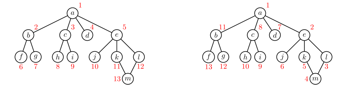
Notice how BFS fans out from vertex a. Every vertex at distance 1 from a is visited before any vertex at distance 2. Then every vertex at distance 2 is visited before any vertex at distance 3. DFS, on the other hand, follows a path down into the graph as far as it can go until it gets stuck. Then it backtracks to its previous location and tries searching from there some more. It continues this strategy of following paths and backtracking.

These are the two key ideas: BFS fans out from the starting vertex, doing a systematic sweep. DFS goes down into the graph until it gets stuck, and then backtracks. If we are just trying to find all the vertices in a graph, then both BFS and DFS will work equally well. However, if we are searching for vertices with a particular property, then depending on where those vertices are located in relation to the start vertex, BFS and DFS will behave differently. BFS, with its systematic search, will always find the closest goal vertex to the starting vertex. However, because of its systematic sweep, it might take BFS a while before it gets to vertices far from the starting vertex. DFS, on the other hand, can very quickly get far from the start, but will often not find the closest vertex first.

The code

Below is some code implementing BFS. It takes a graph and a starting vertex as parameters and returns a set of all the vertices able to be reached from the starting vertex by following paths of vertices and edges.

public static <T> Set<T> bfs(Graph<T> graph, T start) {
    Set<T> found = new LinkedHashSet<T>();
    Deque<T> waiting = new ArrayDeque<T>();
    found.add(start);
    waiting.add(start);

    while (!waiting.isEmpty()) {
        T v = waiting.remove();
        for (T u : graph.getNeighbors(v)) {
            if (!found.contains(u)) {
                found.add(u);
                waiting.add(u);
            }
        }
    }
    return found;
}

We maintain a queue called waiting that contains the vertices in line to be explored, and we maintain a set that contains all the vertices we have found. Initially, both start out with only v in them. We then continually do the following: remove a vertex from the waiting list and loop through its neighbors, adding any neighbor we haven't already found into both the found set and waiting list. The while loop keeps running as long as the waiting list is not empty, i.e. as long as there are still vertices we haven't explored.

A remarkable fact is that the code for DFS is almost exactly the same, except that instead of using a waiting queue, we use a waiting stack. Specifically, the only thing we need to change is to replace waiting.remove with waiting.removeLast. Specifically, the two algorithms differ only in how they choose the next vertex to visit. DFS visits the most recently added vertex, while BFS visits the earliest added vertex.

Let's run BFS on the graph below, starting at vertex a. The first thing the algorithm does is add each of the neighbors of a to the waiting queue. So at this point, the queue is [b,c,d,e]. BFS always visits the first vertex in the queue, so it visits b next and adds its neighbors to the list and set. So now the queue is [c,d,e,f,g]. For the next step, we take the first thing off the queue, which is c and visit it. We add its neighbors h and i to the list and set. This gives us a queue of [d,e,f,g,h,i]. Note also that each time we find a new vertex, we add it to the found set. As the process continues, the queue will start shrinking and the found set will eventually include all the vertices.

Now let's look at the first few steps of DFS on the same graph, starting at vertex a. It starts by adding the neighbors of a to the waiting stack and found. After the first step, the stack is [b,c,d,e]. DFS then visits the last thing on the stack, e, as opposed to BFS, which visits the first. DFS adds the neighbors of e, which are j, k, and l, to the stack, which is now [b,c,d,j,k,l]. It visits the last vertex in the stack, l, and adds its neighbors m and n to the list. This gives a stack of [b,c,d,j,k,m]. We then visit vertex m. It has only one neighbor, k, which has already been found, so we do nothing with that neighbor. This is how we avoid getting stuck in an infinite loop because of the cycle. The stack at this point is now [b,c,d,j,k] and the found set is {a,b,c,d,e,j,k,l,m}. We visit k next. It has a neighbor e, but we don't add e to the stack because e is in the visited set already. The waiting stack is now [b,c,d,j]. The next vertex visited is j. Notice how the algorithm has essentially backtracked to e and is now searching in a different direction from e. The algorithm continues for several more steps from here, but for brevity, we won't include them.

Shortest paths

The searches above find all the vertices that can be reached from a given starting vertex. This is nice, but it is often more useful to be able to find a path between two given vertices. We can take the BFS code above and modify it slightly to find such a path, and because of the way BFS fans out, the path found will be as short as possible. Here is the code:

public static <T> List<T> bfsPath(Graph<T> graph, T start, T end) {
    Deque<T> waiting = new ArrayDeque<T>();
    Map<T, T> parent = new LinkedHashMap<T, T>();

    waiting.add(start);
    parent.put(start,  null);

    while (!waiting.isEmpty()) {
        T v = waiting.remove();
        for (T u : graph.getNeighbors(v)) {
            if (!parent.containsKey(u)) {
                waiting.add(u);
                parent.put(u, v);
            }

            if (u.equals(end)) {
                List<T> path = new ArrayList<T>();
                while (u != null) {
                    path.add(u);
                    u = parent.get(u);
                }
                Collections.reverse(path);
                return path;
            }
        }
    }
    return new ArrayList<T>();
}

What is different here from the BFS code is that instead of a found set, we use a map called parent. Each time we find a new vertex, we record which vertex we reached it from. Once we find the goal vertex, we use that parent map to work our way backward to the start vertex.

Applications of searching

Word ladders

A word ladder is a type of puzzle where you are given two words and you have to get from one to another by changing a single letter at a time, with each intermediate word being a real word. For example, to get from time to rise, we could do time → tide → ride → rise.

We can model this as a graph whose vertices are words, with edges whenever two words differ by a single letter. Solving a word ladder amounts to finding a path in the graph between two vertices. The first thing we will need is a method to determine if two words are one letter away from each other:

public static boolean oneAway(String s, String t) {
    if (s.length() != t.length())
        return false;
    
    int total = 0;
    for (int i=0; i<s.length(); i++)
        if (s.charAt(i) == t.charAt(i))
            total++;
    
    return total == s.length()-1;
}

Now we create the graph. Using a wordlist, we read in all the 4-letter words from the list. Each of those becomes a vertex of the graph. We then use a nested loop to compare each word to each other word and add an edge between any pairs that are one letter apart. This is an O(n²) approach that takes a few seconds to put together the entire graph. It's a nice exercise to try to find a faster approach.^**Hint: Loop over all the words and add an edge to all words that are one letter away. Once the graph is built, we can call the bfsPath method to find the shortest path between two given words, giving us a word ladder between them. Here is the code:

List<String> words = new ArrayList<String>();
Scanner scanner = new Scanner(new File("wordlist.txt"));
while (scanner.hasNext()) {
    String w = scanner.nextLine();
    if (w.length() == 4)
        words.add(w);
}

Graph<String> graph = new Graph<String>();
for (String word : words)
    graph.add(word);

for (int i=0; i<words.size(); i++)
    for (int j=i+1; j<words.size(); j++)
        if (oneAway(words.get(i), words.get(j)))
            graph.addEdge(words.get(i), words.get(j));

System.out.println(bfsPath(graph, "time", "rise"));

Movies

From the International Movie Database (IMDB), it is possible to get a file that contains a rather large number of movies along with the people that have acted in each movie. A fun question to ask is to find a path from one actor X to another Y, along the lines of X acted in a movie with A who acted in a movie with B who acted in a movie with C, etc., until we get to someone who acted in a movie with Y. There are all sorts of things we could study about this, such as whether it is always possible to find such a path or what the length of the shortest path is.

We can model this as a graph where each actor gets a vertex and each movie also gets a vertex. We then add edges between actors and the movies they acted in. The file is structured so that on each line there is a movie name followed by all the actors in that movie. The entries on each line are separated by slashes, like below:

     Princess Bride, The (1987)/Guest, Christopher (I)/Gray, Willoughby/Cook, ...

Here is some code that parses through the file and fills up the graph:

Graph<String> graph = new Graph<String>();
Scanner scanner = new Scanner(new File("movies.txt"));
while (scanner.hasNext()) {
    String line = scanner.nextLine();
    String[] a = line.split("/");
    graph.add(a[0]);
    for (int i=1; i<a.length; i++) {
        graph.add(a[i]);
        graph.addEdge(a[0], a[i]);
    }
}

We can then call bfsPath to find the shortest path between any pair of actors. It turns out that there almost always a path between any two actors that you've ever heard of, and that path is usually pretty short, rarely needing more than a couple of intermediate movies.

Water jug puzzles

Here is an application of digraphs to a classic puzzle problem. Suppose we have two pails, one that holds 7 gallons and another that holds 11 gallons. We have a fountain of water where we can fill up and dump out our pails. Our goal is to get exactly 6 gallons just using these two pails. The rules are that you can only (1) fill up a pail to the top, (2) dump a pail completely out, or (3) dump the contents of one pail into another until the pail is empty or the other is full. There is no guestimating allowed.

For example, maybe we could start by filling up the 7-gallon pail, then dumping it into the 11-gallon pail. We could then fill up the 7-gallon pail and then dump it into the 11-gallon again, leaving 3 gallons in the 7-gallon pail. Maybe then we could dump the 11-gallon pail out completely. We could keep going doing operations like this until we have 6 gallons in one of the pails.

We can represent this problem with a digraph. The vertices are the possible states, represented as pairs (x,y), where x and y are the amount of water in the 7- and 11-gallon pails, respectively. There is an edge between two vertices if it is possible to go from their corresponding states, following the rules of the problem. For example, there is an edge between (3,0) and (0,0) because starting at the (3,0) state, we can dump out the first to get to the (0,0) state. However, there is not an edge going in the opposite direction because there is no way to go from (0,0) to (3,0) in one step following the rules.

To create the graph, we first make a class to represent the states. The class has two integer fields, x and y. We have a simple toString method for the class. We override the equals method because we will need to test states for equality, and we override hashCode because this class is used for vertices, which are themselves keys in a hash map. We have used an IDE to generate these methods. Though the code for this class is long, it is very simple and useful in other places.

private static class Pair {
    private int x;
    private int y;
    
    @Override
    public String toString() {
        return "(" + x + "," + y + ")";
    }

    public Pair(int x, int y) {
        this.x = x;
        this.y = y;
    }

    @Override
    public int hashCode() {
        final int prime = 31;
        int result = 1;
        result = prime * result + x;
        result = prime * result + y;
        return result;
    }

    @Override
    public boolean equals(Object obj) {
        if (this == obj)
            return true;
        if (obj == null)
            return false;
        if (getClass() != obj.getClass())
            return false;
        Pair other = (Pair) obj;
        if (x != other.x)
            return false;
        if (y != other.y)
            return false;
        return true;
    }    
}

Below is the code that creates the digraph. An explanation follows.

Digraph<Pair> G = new Digraph<Pair>();
int M = 7, N = 11;

for (int i=0; i<=M; i++)
    for (int j=0; j<=N; j++)
        G.add(new Pair(i, j));

for (Pair p : G) {
    int x = p.x;
    int y = p.y;
    
    G.addEdge(p, new Pair(0, y));
    G.addEdge(p, new Pair(x, 0));
    G.addEdge(p, new Pair(M, y));
    G.addEdge(p, new Pair(x, N));

    if (x != 0 && y != N) {
        if (x + y > N)
            G.addEdge(p, new Pair(x - (N-y), N));
        else
            G.addEdge(p, new Pair(0, x+y));
    }
    
    if (y != 0 && x != M) {
        if (x + y > M)
            G.addEdge(p, new Pair(M, y - (M-x)));
        else
            G.addEdge(p, new Pair(x+y, 0));
    }
}

System.out.println(bfsPath(G, new Pair(0,0), new Pair(6,0)));

The code starts by adding edges for all the states (0,0), (0,1) up through (M,N). Then for every one of those states we add edges. The first two edges added correspond to emptying out one of the pails. The next two correspond to completely filling up one of the pails.

After that, we have two more edges where we pour one pail into the other. We have to be careful here as doing this will sometimes completely empty one pail and sometimes not, and there is a little math involved to figure out exactly how much will end up in each pail in both cases. We also have to avoid trying to pour into an already full pail or trying to pour from an empty pail.

More applications of graphs

Searching is only one application of graphs. We could easily fill up a book with all the different applications. Here are a few more common applications of graphs:

Social networks

We can model a social network with a graph. The vertices are the people and there is an edge between two vertices if their corresponding people know each other. Questions about the social network, like the average number of people that people know or the average number of connections it takes to get from any one person to another, can be answered by computing properties of the graph.

Scheduling

Suppose we have several people who have to be at certain meetings at a conference. We want to schedule the meetings so that everyone who has to be at a meeting can be there. The main constraint then is that two meetings can't be scheduled for the same time if there is someone who has to be at both. We can represent this as a graph if we let the vertices be the meetings, with an edge between two vertices if there is someone that has to be at both meetings. We then have to assign times to the vertices such that vertices that are connected by an edge must get different times. This is an example of what is called graph coloring and it can be used to model a lot of problems like this. If we implement an algorithm to find proper colorings of graphs, then all we have to do is represent our real-life problem with a graph and then run the algorithm on that.

Shortest paths

An important type of graph is a weighted graph, where the edges have numerical values called weights attached to them. Suppose we have a graph where the vertices are locations and the edges are roads connecting them. Weights could be the costs of using those roads, in terms of time, distance, or money. We would then be interested in the shortest or cheapest path between two vertices. The shortest path algorithm is a relative of the BFS algorithm we wrote earlier. This, or something like it, is used by GPS systems to find directions.

Spanning trees

A spanning tree of a graph is a subgraph that is a tree and contains all the vertices. Spanning trees are useful in routing packets over a network. Networks can often be complicated and it's possible to get a routing loop, where a packet gets caught in a loop and never gets to its destination. By finding a spanning tree in a network, we get a subgraph that still connects all the vertices but contains no cycles, which will allow us to prevent routing loops.

Matchings

An important type of problem is a bipartite matching, where we have two groups of vertices along with edges from some vertices in one group to some in the other group, with those edges indicating which vertices in the one group are compatible with those in the other. We are interested in matching as many possible vertices in the one group with vertices in the other.

Network flows

Imagine we have a weighted graph representing a transportation network where the weights on the edges represent capacities for how much stuff we can push through those edges. We are interested in maximizing the flow so that we can get as much stuff from a designated source vertex to a designated sink vertex.

Most books on graph theory or on algorithms will have details on these problems and many more.

Sorting

Introduction

This chapter is about a variety of algorithms for sorting arrays and lists. Most higher level languages have sorting built in to the language (for instance, Java has Collections.sort and Arrays.sort), so it not as useful now to know how to sort things as it once was, when programmers often had to implement their own sorts. However, it is still useful to know how some of the different sorts work. It is also good practice to implement the algorithms. Knowledge of these things is considered foundational computer science knowledge, and moreover, some of the ideas behind the algorithms are useful in other situations. A few notes:

We will implement all the searches on integer arrays instead of on generic lists. The reason for this is that array syntax is simpler and more readable than list syntax. In practice, though, it is usually better to use lists in place of arrays. It is not hard to translate the array algorithms to list algorithms. This is covered in Section 11.7.
For clarity, the figures demonstrating the sorts will use letters instead of numbers.
Our sorts will directly modify the caller's array. We could also leave the array untouched and return a new sorted array, but we've chosen this approach for simplicity.

The first three sorts that we cover—insertion sort, mergesort, and quicksort—are arguably the three most important sorts. The other sorts we cover are nice to know, but not as important as the these three.

Insertion sort

Insertion sort is an O(n²) sorting algorithm. It is slower than mergesort and quicksort for large arrays, but it is simple and faster than those sorts for very small arrays (of size up to maybe a few dozen elements). Mergesort and quicksort require a certain amount of setup work or overhead due to recursion that insertion sort doesn't. Once they get going, however, they will usually outperform insertion sort.

To understand the basic idea, suppose we have a stack of papers we want to put into in alphabetical order. We could start by putting the first two papers in order. Then we could put the third paper where it fits in order with the other two. Then we could put the fourth paper where it fits in order with the first three. If we keep doing this, we have what is essentially insertion sort.

To do insertion sort on an array, we loop over the indices of the array running from 1 to the end of the array. For each index, we take the element at that index and loop back through the array towards the front, looking for where the element belongs among the earlier elements. These elements are in sorted order (having been placed in order by the previous steps), so to find the location we run the loop until we find an element that is smaller than the one we or looking at or fall off the front of the array. The figure below shows it in action.

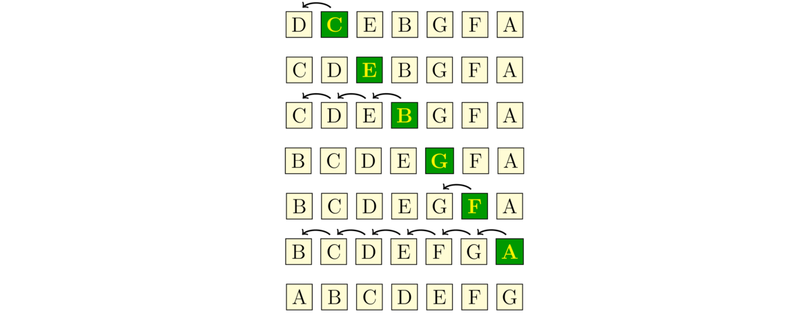
Here is the code:

public static void insertionSort(int[] a) {
    for (int i=1; i<a.length; i++) {
        int hold = a[i];
        int j = i;
        while (j>=1 && a[j-1]>hold) {
            a[j] = a[j-1];
            j--;
        }
        a[j] = hold;    
    }
}

The outer loop goes through each new element of the array, and the inner determines where to place that element.

We see the nested loops in the code, which is where the O(n²) running time comes from. If the list is already sorted, the condition on the inner while loop will always be false and insertion sort runs in O(n) time, which is the best any sorting algorithm can manage. In fact, insertion sort can run relatively quickly even on very large arrays if those arrays are nearly sorted. On the other hand, if the list is in reverse order, the while loop condition is always true and we have n(n-1)/2 swaps, which is about as bad as things can get for a sort.

Mergesort

Mergesort is one of the fastest sorts available. It runs in O(n log n) time for all inputs. The sorting algorithms built into many programming languages (including Java) use mergesort or a variation of it called timsort.

Mergesort works as follows: We break the array into two halves, sort them, and then merge them together. The halves themselves are sorted with mergesort, making this is a recursive algorithm. For instance, say we want to sort the string CEIGJBFDHA. We break it up into two halves, CEIGJ and BFDHA. We then sort those halves (using mergesort) to get CEGIJ and ABDFH and merge the sorted halves back together to get ABCDEFGHIJ. See the figure below:

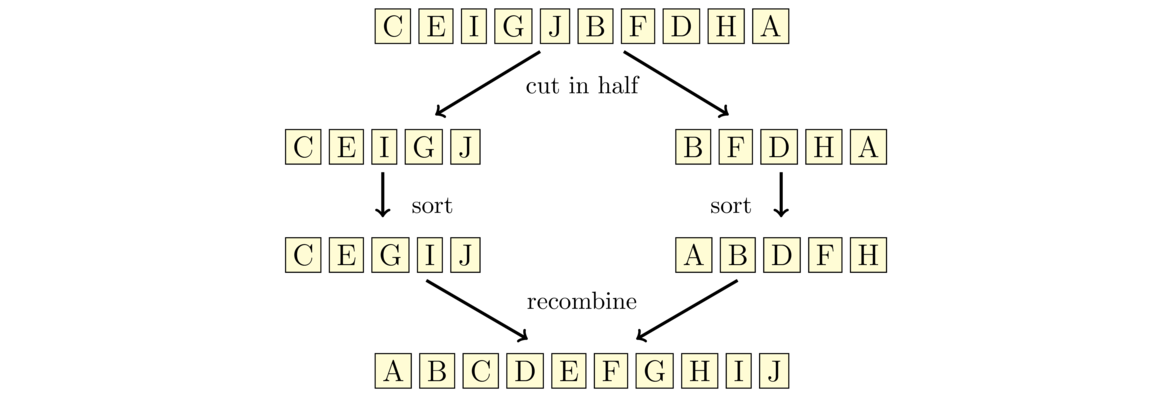
The way the merging process works is we have position markers (counters) for each of the two halves, each initially at the starts of their corresponding halves. We compare the values at the markers, choose the smaller of the two, and advance the corresponding marker. We repeat the process until we reach the end of one of the halves. After that, we append any remaining items from the other half to the end. The first few steps are shown below:

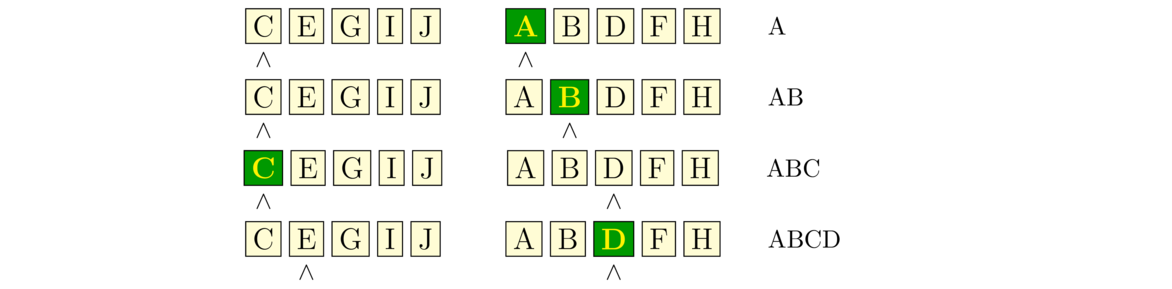
Here is the code for mergesort:

public static void mergesort(int[] a) {
    if (a.length <= 1)
        return;

    int[] left  = Arrays.copyOfRange(a, 0, a.length/2);
    int[] right = Arrays.copyOfRange(a, a.length/2, a.length);
        
    mergesort(left);
    mergesort(right);

    int[] m = merge(left, right);
    for (int i=0; i<a.length; i++)
        a[i] = m[i];
}

private static int[] merge(int[] a, int[] b) {
    int[] m = new int[a.length + b.length];
    int x=0, y=0, z=0;
    
    while (x < a.length && y < b.length) {
        if (a[x] < b[y])
            m[z++] = a[x++];
        else
            m[z++] = b[y++];
    }
    
    while (x < a.length)
        m[z++] = a[x++];        
    while (y < b.length)
        m[z++] = b[y++];

    return m;
}

After the base case, the mergesort method breaks the list into its left and right halves using the Arrays.copyOfRange method. It then recursively calls mergesort on those two halves and calls the merge method to put things back together. At the end we copy the result back into the a variable, overwriting the old array with the new, sorted one.

The merge method first declares a new array that will hold the merged result and it sets up counters x, y that are the position markers mentioned above. The counter z is to keep track of what index we are adding to in the m array. We then loop until one of the counters x and y reaches the end of its array. In that loop, we compare the array values at those indices and put the smaller one into the m array. After the loop, if there is anything left in either a or b, will add all of it to the end of m.

One thing to note is that to keep the code short, we use the ++ operator. When used like this, the incrementing happens after the assignment. So, for instance, the code on the left is equivalent to the code on the right.

m[z++] = a[x++];                 m[z] = a[x];
                                 z++;
                                 x++;

Not everyone likes this way of doing things, but some people do and you will likely see it in the future, especially if you work with C or C++.

This version of mergesort is a little slow. There are several places that it can be improved, but one in particular stands out—we waste a lot of time creating new arrays. Creating and filling a new array is time-consuming, and we create three new arrays with each recursive call of the function. There is a way around this that involves doing most of the sorting and merging within the original array. We will need to create just one other array, b, with the same size as a as a place to temporarily store some things when merging. The key is that instead of creating the left and right arrays, we will work completely within a, using indices called left, mid, right to keep track of where in the array we are currently sorting. These become parameters to the merge function itself. The faster code is below:

public static void mergesort(int[] a) {
    int[] b = new int[a.length];
    mergesortHelper(a, b, 0, a.length);
}

private static void mergesortHelper(int[] a, int[] b, int left, int right) {
    if (right-left <= 1)
        return;
    
    int mid = (left + right) / 2;
    mergesortHelper(a, b, left, mid);
    mergesortHelper(a, b, mid, right);
    
    for (int i=left; i<right; i++)
        b[i] = a[i];
    
    int x=left, y=mid, z=left;
    while (x < mid && y < right) {
        if (b[x] < b[y])
            a[z++] = b[x++];
        else
            a[z++] = b[y++];
    }

    while (x < mid)
        a[z++] = b[x++];
    while (y < right)
        a[z++] = b[y++];
}

If you look closely, you'll see that the structure of this code really is the same as what we wrote earlier, just reworked to avoid continually creating arrays.

Mergesort runs in O(n log n) time. Unlike many other sorting algorithms, mergesort is pretty consistent in that it runs in O(n log n) time for all inputs. There really aren't any inputs that it does really well with or really poorly with.

Quicksort

Quicksort is one of the fastest sorting algorithms. It is built into a number of programming languages. Like mergesort, it works by breaking the array into two subarrays, sorting them and then recombining.

Quicksort first picks an element of the array to serve as a pivot. For simplicity, we will use the first element. Quicksort then breaks the array into the portion that consists of all the elements less than or equal to the pivot and the portion that consists of all the elements greater than the pivot. For instance, if we are sorting CEIGJBFDHA, then the pivot is C, and the two portions are BA (everything less than the pivot) and EIGJFDH (everything greater than the pivot).

We then sort the two portions using quicksort again, making this a recursive algorithm. Finally, we combine the portions. Because we know that all the things in the one portion are less than or equal to the pivot and all the things in the other portion are greater than the pivot, putting things together is quick. See the figure below:

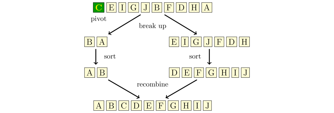
Notice that the way quicksort breaks up the array is more complicated way than the way mergesort does, but then quicksort has an easier time putting things back together than mergesort does. Here is the quicksort code:

public static void quicksort(int[] a) {    
    if (a.length <= 1)
        return;
    
    int[] smaller = new int[a.length-1];
    int[] larger = new int[a.length-1];
    int pivot = a[0];
    
    int d = 0, e = 0;
    for (int i=1; i<a.length; i++) {
        if (a[i] <= pivot)
            smaller[d++] = a[i];
        else
            larger[e++] = a[i];
    }
    smaller = Arrays.copyOf(smaller, d);
    larger = Arrays.copyOf(larger, e);
    
    quicksort(smaller);
    quicksort(larger);
    
    int c = 0;
    for (int x : smaller)
        a[c++] = x;
    a[c++] = pivot;
    for (int x : larger)
        a[c++] = x;
}

After the base case, the code creates two arrays to hold the things less than or equal to the pivot and the things greater than the pivot. We then loop through the main array to fill up these two arrays. We initially don't know how large to make the two arrays, so we set their initial sizes to a.length-1 and then use Arrays.copyOf to resize them to their correct sizes. After this, we call quicksort recursively and then combine the two parts along with the pivot into the final, sorted result.

There is a problem with our implementation—contrary to its name, our algorithm is slow. Creating the subarrays is very time-consuming, particularly because we create two new arrays, recopy them, and then put them back together. And this happens with each recursive call of the function. We can get a considerable speedup by doing the partition in-place. That is, we will not create any new arrays, but instead we will move things around in the main array. This is not unlike how we sped up our mergesort implementation.

We use two indices, i and j, with i starting at the left end of the array and j starting at the right. Both indices move towards the middle of the array. We first advance i until we meet an element that is greater than or equal to the pivot. We then advance j until we meet an element that is less than or equal to the pivot. When this happens, we swap the elements at each index. We then continue advancing the indices and swapping in the same way, stopping the process once the once the i and j indices meet each other. See the figure below:

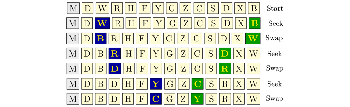
In the figure above, the pivot is M, the first letter in the array. The figure is broken down into “seek” phases, where we advance i and j, and swap phases, where we exchange the values at those indices. The blue highlighted letter on the left corresponds to the position of i and the green highlighted letter on the right corresponds to the position of j. Notice at the last step how they cross paths.

This process partitions the array. We then make recursive calls to quicksort, using the positions of the indices i and j to indicate where the two subarrays are located in the main array. In particular, we make a recursive call on the subarray starting at the left end and ending at the position of i, and we make a recursive call on the subarray starting at the position of j and ending at the right end. So in the example above, we would call quicksort on the subarrays from 0 to 8 and from 8 to 13. Here is the code for our improved quicksort:

public static void quicksort(int[] a) {
    quicksort_helper(a, 0, a.length-1);
}

public static void quicksort_helper(int[] a, int left, int right) {
    if (left >= right)
        return;

    int i=left, j=right, pivot=a[left];
    while (i <= j) {
        while (a[i] < pivot)
            i++;
        while (a[j] > pivot)
            j--;
        if (i <= j) {
            int hold = a[i];
            a[i++] = a[j];
            a[j--] = hold;
        }
    }    
    quicksort_helper(a, i, right);
    quicksort_helper(a, left, j);
}

Quicksort generally has an O(n log n) running time, but there are some special cases where it degenerates to O(n²). One of these would be if the array was already sorted. In that case the subarray smaller will be empty, while the subarray larger will have size n-1. When we call quicksort on larger, we will again have the same problem with the new smaller array being empty and the new larger array having size n-2. This will continue with the larger array going down in size by 1 at each step. This will lead to n recursive calls, each taking O(n) time, so we end up with an O(n²) running time overall. Since real-life arrays are often sorted or nearly so, this is an important problem. One way around this problem is to use a different pivot, such as one in the middle of the array or one that is chosen randomly.

Other sorts

There are dozens of important sorting algorithms besides the ones we have already looked at. In this section we will look at a few of them.

Selection sort

Selection sort is one of this simplest sorts to implement, but it is also slow. It works as follows: Start by considering the first element of the array in relation to all the other elements. Find the smallest element among the others and if it is less than the first element, then swap them. Now move on to the second element of the array. Look at all the elements after the second, find the smallest element among them, and if it is smaller than the second element, then swap them. We continue the same process for the third, fourth, etc. elements in the array, until we reach the end.

This method is so slow that it is not really worth using except that a variation of it is extremely quick to implement, consisting of nested loops, a comparison, and a swap, as shown below:

public static void selectionSortVariant(int[] a) {
    for (int i=0; i<a.length-1; i++) {
        for (int j=i+1; j<a.length; j++) {
            if (a[i] > a[j]) {
                int hold = a[i];
                a[i] = a[j];
                a[j] = hold;
            }
        }
    }
}

Bubble sort

Bubble sort is a relative of selection sort. It is also extremely slow. We include it here only because it's probably the most famous sorting algorithm.

We start at the end of the array and compare the last and second-to-last elements, swapping if necessary. We then compare the second-to-last element with the third-to-last. Then we compare the third-to-last with the fourth-to-last. We keep going in this way until we reach the front of the array. At this point, the first position in the array will be correct. The correct element “bubbles up” to the front of the array. We then start at the end of the array and repeat the process, but this time instead of going all the way to the front, we stop at the second element (because we know the first element is already correct). After this stage, the second element is correct.

We then continue the process, where at each step, we start at the end of the array and compare adjacent elements and continue doing that until we get to the stopping point. At each step, the stopping point moves one index forward until we reach the end of the array. The figure below shows the order in which elements are compared. The arrows indicate when a swap is performed.

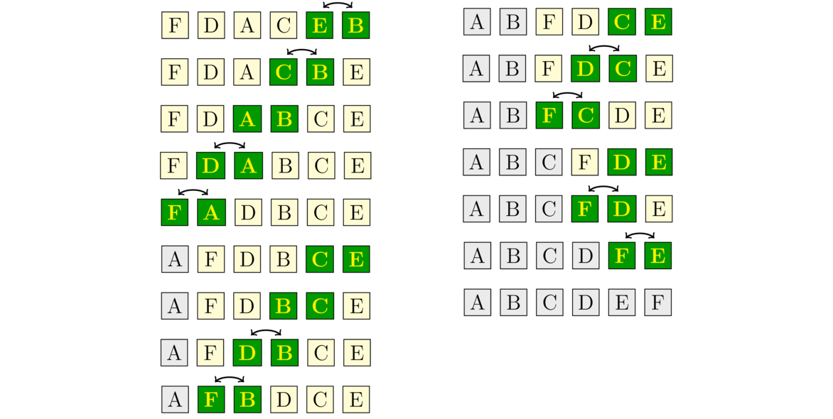
We use nested for loops to implement the algorithm. The outer loop keeps track of the stopping point. It starts at the front of the array and works its way toward the end. The inner loop always starts at the end of the array and ends at the stopping point. Inside the loop we compare adjacent elements and swap if necessary.

public static void bubbleSort(int[] a) {
    for (int i=0; i<a.length-1; i++) {
        for(int j=a.length-1; j>i; j--) {
            if (a[j-1] > a[j]) {
                int hold = a[j-1];
                a[j-1] = a[j];
                a[j] = hold;
            }
        }
    }
}

Just like selection sort, bubble sort is O(n²), making n(n-1)/2 comparisons, regardless of whether the array is already sorted or completely jumbled. However, we can actually improve on this. If there are no swaps made on one of the passes through the array (i.e., one run of the inner loop), then the array must be sorted and we can stop. This improvement, however, is still not enough to make bubble sort useful for sorting large arrays. In fact, its performance can be worse than the ordinary bubble sort for large, well-mixed arrays. .

Shellsort

Shellsort builds on insertion sort. Here is an example of one variation of shellsort: We start by pulling out every fourth character starting with the first and using insertion sort to sort just those characters. We then pull out every fourth character starting with the second character and use insertion sort to sort those characters. We do the same for every fourth character starting with the third and then every fourth starting with the fourth. See the figure below:

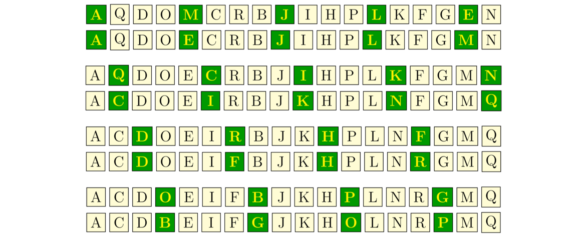
We then do something similar except we break up the array at a finer scale, first breaking it up at every second character starting with the first, sorting those characters, and then breaking it up at every second character starting with the second and sorting, as shown below:

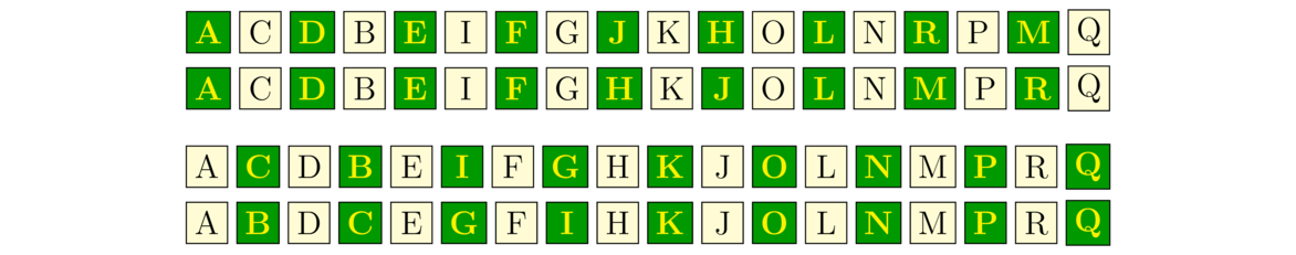
At this point the array is nearly sorted.

We run a final insertion sort on the entire array to sort it. This step is pretty quick because only a few swaps need to be made before the array is sorted. Now it may seem like we did so many individual sorts that it would have been more efficient to just have run a single insertion sort in the first place, but that is not the case. The total number of comparisons and swaps needed will often be quite a bit less for shellsort than for insertion sort.

In the example above, we used gaps of length 4, 2, and 1. The sequence (4,2,1) is called a gap-sequence. There are a variety of different gap sequences one could use, the only requirement being that the last gap is 1. An implementation of shellsort is shown below using a very specific gap sequence. The code is surprisingly short and very efficient as it essentially works on all the subarrays for a given gap at once. In the example above, with a gap of 4, we did four separate steps, but the code below would handle them all together.

public static void shellsort(int[] a) {
    int[] gaps = {1391376, 463792, 198768, 86961, 33936, 13776, 4592,
                  1968, 861, 336, 112, 48, 21, 7, 3, 1};

    for (int gap : gaps) {
        for (int i=gap; i<a.length; i++) {
            int hold = a[i];
            int j = i;
            while (j >= gap && a[j-gap] > hold) {
                a[j] = a[j-gap];
                j-=gap;
            }
            a[j] = hold;
        }
    }
}

Different gap sequences produce different running times. Some produce an O(n²) running time, while others can get somewhat closer to O(n), with running times like O(n^5/4) or O(n^3/2). Determining the running time for a given gap sequence can be tricky. In fact, the running times for some popular gap sequences are unknown. People are even now still looking for better gap sequences. Shellsort is not quite as popular as mergesort or quicksort, but it is a nice sort with performance comparable to those algorithms in a few specific applications.

Heapsort

Heapsort uses a heap to sort an array. Recall that a heap is a data structure that gives easy access to the smallest item. Using a heap to sort an array is very easy—we just run through the array, putting the elements one-by-one onto the heap and when that's done, we then one-by-one remove the top element from the heap. Since the top item of a heap is always the smallest item, things will come out in sorted order.

The PriorityQueue class in Java's Collections Framework is implemented using a heap. So we can use Java's PriorityQueue to implement heapsort. Here is the code:

public static void heapsort(int[] a) {
    PriorityQueue<Integer> heap = new PriorityQueue<Integer>();
    
    for (int i=0; i<a.length; i++)
        heap.add(a[i]);
    
    for (int i=0; i<a.length; i++)
        a[i] = heap.remove();
}

Heapsort has an O(n log n) running time. When we insert the elements into the heap we have to loop through the array, so that's where the n comes from. Adding each element to the heap is an O(log n) operation, so overall adding the elements of the array into the heap takes O(n log n) time. Looping through and removing the items also takes O(n log n) time. Heapsort is one of the faster sorts. It runs in O(n log n) time regardless of whether the data is already sorted, in reverse order, or whatever.

A close relative of heapsort is treesort that works in the same way but uses a BST in place of a heap.

Counting sort

If we know something about the data in our array, then we can do better than the O(n log n) algorithms we've seen. For instance, if we know that we know the array contains only values in a relatively small range, then we can use an O(n) sort known as counting sort.

Counting sort works by keeping an array of counts of how many times each element occurs in the array. We scan through the array and each time we meet an element, we add 1 to its count. Suppose we know that our arrays will only contain integers between 0 and 9. If we have the array [1,2,5,0,1,5,1,3,5], the array of counts would be [1,3,1,1,0,3,0,0,0,0] because we have 1 zero, 3 ones, 1 two, 1 three, no fours, 3 fives, and no sixes, sevens, eights, or nines.

We can then use this array of counts to construct the sorted list [0,1,1,1,2,3,5,5,5] by repeating 0 one time, repeating 1 three times, repeating 2 one time, etc., starting from 0 and repeating each element according to its count. Here is code for the counting sort. The max argument needs to be at least as large as the largest thing in the array.

public static void countingSort(int[] a, int max) {
    int[] counts = new int[max + 1];
    
    for (int x : a)
        counts[x]++;
    
    int c=0;
    for (int i=0; i<counts.length; i++)
        for (int j=0; j<counts[i]; j++)
            a[c++] = i;
}

This simple sort has an O(n) running time. The only drawback is that it only works if the array consists of integers between 0 and max. This approach becomes infeasible if max is very large.

Comparison of sorting algorithms

First, mergesort and quicksort are considered to be the fastest sorts. Insertion sort can be better than those on small arrays (up to maybe a few dozen elements, depending on a variety of factors). Heapsort is competitive with mergesort and quicksort, but is not quite as fast. Shellsort can be competitive with these sorts in a few specific applications. Counting sort is faster than all of them but works best with values in a limited range. Selection sort and bubble sort are mostly of historical interest.

In terms of asymptotics, the running time of a sort must always be at least O(n) because you have to look at every element before you know if the array is sorted. We have seen that counting sort achieves the O(n) optimum. Also, it can be shown that any sort that works by comparing one element to another must have a running time of at least O(n log n). The O(n log n) sorts that we have seen are heapsort, mergesort, and quicksort.

Regarding the big O running times, remember that there are constants involved. For instance, selection sort and bubble sort are both O(n²) algorithms, but it may turn out that selection sort's running time is something like 10n² and bubble sort's is 15n², making selection sort a bit faster. These values of 10 and 15 are made up, but the point is that there are constants in the running times that do not appear in the big O notation, and those constants are important in the overall running time.

A bit more practically, the O(n²) insertion sort beats the O(n log n) mergesort for small arrays. This could happen if insertion sort's running time looks something like 0.2n² and mergesort's running time looks like 2n log n. For values up until around 50, 0.2n² is smaller, but after n=50 the n² term starts to dominate n log n. So in this scenario, insertion sort is faster than mergesort up through around n=50.

There is more to the story than just big O. One thing that matters is exactly how the algorithms are implemented and on what sort of data they will be used. For instance, working with integer arrays where comparisons are simple is a lot different than working on arrays of objects where the comparison operation might be fairly complex. Similarly, swapping integers is quicker than swapping objects. So in certain situations a sorting algorithm that uses less comparisons or less swaps may be better.

Another consideration is memory usage. Most of the O(n log n) algorithms have memory usage associated with either a data structure, recursive overhead, or using auxiliary arrays to hold intermediate results.

Also, we need to consider how the algorithms work with memory. For instance, it is important whether the algorithm reads from memory sequentially or randomly. This is important, for example, when sorting large files that require reads from a hard disk drive. Repositioning the read head on a hard disk is slow, whereas once it is positioned, reading the next elements in sequence is relatively fast. So, since mergesort does sequential reads and quicksort does random ones, mergesort may be better when a lot of reading from a hard disk is required. Some of these same considerations apply to how well the algorithm makes use of cache memory.

Another important consideration is whether the algorithm is stable or not. This concept comes in when sorting objects based on one of their fields. For example, suppose we have a list of person objects with fields for name and age, and we are sorting based on age. Suppose entries in the list are already alphabetized. A stable sort will maintain the alphabetical order while sorting by age, whereas an unstable one may not. Of the sorts we have looked at, bubble sort, insertion sort, and mergesort are stable, while selection sort, shellsort, heapsort, and quicksort are not, though some of them can be modified to be stable.

One last practical consideration is that real-life data often has some structure to it. For instance, timsort, a variation of mergesort, takes advantage of the fact that real-life data there are often pockets of data, called runs, that are sorted or nearly so within the larger array.

There are still further considerations that we won't get into here. In summary, each of the algorithms has its good and bad points, but of all the algorithms, quicksort and mergesort are probably the most used.

Summary of running times

Here is a table of the running times of the sorts:

	Average	Worst	Already sorted
Selection	O(n²)	O(n²)	O(n²)
Bubble	O(n²)	O(n²)	O(n²)^*
Insertion	O(n²)	O(n²)	O(n)
Shell^†	varies	varies	varies
Heap	O(n log n)	O(n log n)	O(n log n)
Merge	O(n log n)	O(n log n)	O(n log n)
Quick	O(n log n)	O(n²)	O(n log n)^‡
Counting	O(n)	O(n)	O(n)

[*] An easy modification makes this O(n).
[†] The results for shellsort vary depending on the gap sequence. For some gap sequences, the worst-case running time is O(n²), O(n^4/3) or even O(n log² n). The average case running times for most gap sequences used in practice are unknown. For already sorted data, the running time can be O(n log n) or O(n), depending on the gap sequence.
[‡] Depends on the pivot. Choosing the first element as the pivot will make this O(n²), but choosing the middle element will make it O(n log n).

Finally, to close out the section, we have a comparison of the sorting algorithms from this chapter. I ran each sorting algorithm on the same 100 randomly generated arrays consisting of integers from 0 to 99999 for a variety of sizes from 10 through 10,000,000. This is mostly for fun and is not meant to be a scientific study. Here are the results. Times are given in milliseconds.

10		100		1000		10,000		100,000		1,000,000		10,000,000
Insert	0.0032	Quick	0.013	Quick	0.11	Count	0.4	Count	1.6	Count	6	Count	47
Quick	0.0043	Merge	0.026	Merge	0.17	Quick	1.1	Quick	12.2	Quick	125	Quick	1107
Select	0.0055	Insert	0.052	Shell	0.18	Shell	1.4	Shell	15.2	Merge	167	Merge	1791
Merge	0.0116	Shell	0.078	Count	0.32	Merge	1.5	Merge	15.3	Shell	182	Shell	2010
Shell	0.0156	Select	0.107	Insert	0.37	Heap	2.1	Heap	28.8	Heap	765	Heap	12800
Bubble	0.0211	Bubble	0.115	Heap	0.39	Insert	20.1	Insert	1963.2	Insert*		Insert*
Heap	0.0390	Heap	0.117	Select	0.89	Select	50.2	Select	4854.0	Select*		Select*
Count	0.3631	Count	0.413	Bubble	1.73	Bubble	157.6	Bubble	18262.3	Bubble*		Bubble*

* Not attempted because they would take too long

Notice in particular, the difference between the O(n) counting sort, the O(n log n) heapsort, mergesort, and quicksort, and the O(n²) selection sort, bubble sort, and insertion sort. The difference is especially clear for n= 100,000.

Here are the results sorted by algorithm:

	10	100	1000	10,000	100,000	1,000,000	10,000,000
Bubble	0.0211	0.115	1.73	157.6	18262.3
Count	0.3631	0.413	0.32	0.4	1.6	6	47
Heap	0.0390	0.117	0.39	2.1	28.8	765	12800
Insert	0.0032	0.052	0.37	20.1	1963.2
Merge	0.0116	0.026	0.17	1.5	15.3	167	1791
Quick	0.0043	0.013	0.11	1.1	12.2	125	1107
Select	0.0055	0.107	0.89	50.2	4854.0
Shell	0.0156	0.078	0.18	1.4	15.2	182	2010

The tests for large arrays were not run on insertion sort, bubble sort, or selection sort because they would take far too long. In fact, when looking at the times for these algorithms, we can see the O(n²) growth. Look, for instance, at the bubble sort times. We see that as n goes from 100 to 1000 (up by a factor of 10), the time goes from .115 to 1.73, an increase of roughly 100 times. From n=1000 to 10000 we see a similar near hundredfold increase from 1.73 to 157.6. From n=10000 to 100000, it again goes up by a factor of nearly 100, from 157.6 to 18262.3. This is quadratic growth —a tenfold increase in n translates to a hundredfold (100=10²) increase in running time. Were we to try running bubble sort with n=1,000,000, we would expect a running time on the order of about 2000000 milliseconds (about 30 minutes). At n=10,000,000, bubble sort would take about 3000 minutes (about 2 days).

Sorting in Java

Sorting with generics and lists

As mentioned, we wrote the sorting methods to work just on integer arrays in order to keep the code simple, without too much syntax getting in the way. It's not too much work to modify the methods to work with other data types. We use lists instead of arrays and use generics to support multiple data types.

Here is the variation on the selection sort algorithm on an integer array from Section 11.5:

public static void selectionSortVariant(int[] a) {
    for (int i=0; i<a.length-1; i++) {
        for (int j=i+1; j<a.length; j++) {
            if (a[i] > a[j]) {
                int hold = a[i];
                a[i] = a[j];
                a[j] = hold;
            }
        }
    }
}

Here is its modification to run with a list of objects:

public static <T extends Comparable<T>> void selectionSortVariant(List<T> a) {
    for (int i=0; i<a.size()-1; i++) {
        for (int j=i; j<a.size(); j++) {
            if (a.get(i).compareTo(a.get(j)) > 0) {
                T hold = a.get(i);
                a.set(i, a.get(j));
                a.set(j, hold);
            }
        }
    }
}

This will run on any data type that implements the Comparable interface, i.e. any data type for which a way to compare elements has been defined. This includes, integers, doubles, strings, and any user-defined classes for which comparison code using the Comparable interface has been written.

Java's sorting methods

There is an array sorting method in java.util.Arrays. Here is an example of it:

int[] a = {3,9,4,1,3,2};
Arrays.sort(a);

When working with lists, one approach is Collections.sort. Here is an example:

List<Integer> list = new ArrayList<Integer>();
Collections.addAll(list, 3,9,4,1,3,2);
Collections.sort(list);

In Java 8 and later, lists now have a sorting method, as shown below:

List<Integer> list = new ArrayList<Integer>();
Collections.addAll(list, 3,9,4,1,3,2);
list.sort();

Sorting by a special criterion

Sometimes, we have objects that we want to sort according to a certain rule. For example, it is sometimes useful to sort strings by length rather than alphabetically. In Java 7 and earlier, the syntax for these things is a little complicated. Here is the old way to sort an array of strings by length:

Collections.sort(list, new Comparator<String>() {
    public int compare(String s, String t) {
        return s.length() - t.length(); }});

This uses something called a Comparator. The key part of it is a function that tells how to do the comparison. That function works like the compareTo method of the Comparable interface in that it returns a negative, 0, or positive depending on whether the first argument is less than, equal to, or greater than the second argument. The example above uses an anonymous class. It is possible, but usually unnecessary, to create a separate, standalone Comparator class.

Things are much easier in Java 8. Here is code to sort a list of strings by length:

list.sort((s,t) -> s.length() - t.length());

In place of an entire anonymous Comparator class, Java 8 allows you to specify an anonymous function. It basically cuts through all the syntax to get to just the part of the Comparator's compare function that shows how to do the comparison.

Sorting by an object's field

Here is another example. Say we have a class called Record that has three fields—firstName, lastName, and age—and we want to sort a list of records by age.

We could use the following:

Collections.sort(list, new Comparator<Record>() {
    public int compare(Record r1, Record r2) {
        return r1.age - r2.age; }});

In Java 8, we can do the following:

list.sort((r1, r2) -> r1.age - r2.age);

If we have a getter written for the age, we could also do the following:

list.sort(Comparator.comparing(Record::getAge));

Suppose we want to sort by a more complicated criterion, like by last name and then by first name. The following is one way to do things:

Collections.sort(list, new Comparator<Record>() {
            public int compare(Record r1, Record r2) {
                if (!r1.lastName.equals(r2.lastName))
                    return r1.lastName.compareTo(r2.lastName);
                else
                    return r1.firstName.compareTo(r2.firstName); }});

In Java 8, we can use the following:

list.sort(Comparator.comparing(Record::getLastName).thenComparing(Record::getFirstName));

Exercises

Chapter 1 Exercises

Order the running times below from slowest to fastest:

O(log n), O(2ⁿ), O(1), O(n), O(n²), O(n³), O(n log n),
The running time certain algorithms has been determined to be exactly the values given below. Using big O notation, how would people usually write these (in their simplest possible form)?
1. n²+2n+3
2. 3+5n²
3. 4.034n³+2.116n+9.037
4. 24n+10n⁴+270.09
5. n+log n
6. 100 · 2ⁿ + n!/5
Suppose we have an algorithm that takes a list of size n as its only parameter. Regardless of the value of n, the algorithm takes 45 seconds to run. Fill in the blank: This is an O( ) algorithm.
Suppose we have a list of 1 quadrillion names (that's 10¹⁵ names) sorted alphabetically. We are searching the list to see if a particular name appears.
1. If we do a linear search, in the worst case scenario, how many names will we need to individually examine before we can determine if the name is in the list or not?
2. If we do a binary search, in the worst case scenario, how many names will we need to individually examine before we can determine if the name is in the list or not?
Is an O(n) algorithm always better than an O(n²) algorithm? Explain, preferably using an example.

Give the asymptotic running time of the following segments of code using big O notation in terms of n=a.length.

int count = 0;
for (int i=0; i<a.length; i++)
    count++;

int sum=0;
for (int i=0; i<a.length; i++) {
    for (int j=0; j<a.length; j++) {
        for (int k=0; k<a.length; k++)
            sum += a[i]*a[j]*a[k];
    }
}

int sum=0;
for (int i=0; i<10; i++) {
    for (int j=0; j<a.length; j++) {
        for (int k=0; k<10; k++)
            sum += a[i]*a[j]*a[k];
    }
}

int i = 1;
while (i < a.length) {
    System.out.println(a[i]);
    i *= 2;
}

if (a.length < 2)
    System.out.println("Too small.");
else if (a.length > 100)
    System.out.println("Too large.");
else
    System.out.println(a[a.length-1]);

for (int i=0; i<a.length; i++) {
    for (int j=0; j<a.length; j++)
        System.out.println(a[i] - a[j]);

    for (int j=0; j<a.length; i++)
        System.out.print(a[j] - a[i]);
}

for (int i=a.length-1; i>0; i/=2)
    a[i] = 0;

int i = a.length-1;
while (i >= 1) {
    int j=0;
    while (j < a.length) {
        a[j]+=i;
        j++;
    }
    i /= 2;
}

int sum=0;
for (int i=0; i<a.length; i++)
    for (int j=0; j<a.length; j++)
        for (int k=0; k<a.length; k++)
            for (int m=0; m<a.length; m++)
                sum += a[i]/a[j]+a[k]/a[m];

int s = 0;
for (int i=0; i<100; i++)
    sum += a[i];

int i = a.length-1;
while (i >= 1) {
    System.out.println(a[i]);
    i /= 3;
}

for (int i=0; i<a.length; i++) {
    for (int j=0; j<a.length; j++)
    System.out.println(a[i] + a[j]);
}

for (int i=0; i<a.length; i++)
    System.out.print(a[i] + " ");

int i = a.length-1;
while (i>=1) {
    for (int j=0; j<a.length; j++)
        a[j]+=i;
    i /= 3;
}

for (int i=1; i<a.length; i *= 2)
    a[i] = 0;

int sum = 0;
for (int i=0; i<a.length; i++) {
    for (int j=0; j<a.length; j += 2)
        sum += a[i]*j;
}

int sum = 0;
for (int i=0; i<a.length; i++) {
    for (int j=0; j<100; j += 2)
        sum += a[i]*j;
}

int sum = 0;
System.out.println((a[0]+a[a.length-1])/2.0);

int sum = 0;
for (int i=0; i<a.length; i++) {
    int j = 0;
    while (j < a.length) {
        for (int k=0; k<a.length; k++)
            sum += a[i]*j;
        j++;
    }
}

for (int i=0; i<1000; i++)
    System.out.println(Math.pow(a[0], i));

int i = 1;
while (i < a.length) {
    a[i] = 0;
    i *= 2;
}

for (int i=0; i<a.length; i++)
    System.out.println(a);

Chapter 2 Exercises

If we create an AList object, add values into it so it equals [1, 3, 6, 10, 15] and then call the f method, what will the list look like after the call?
```
public void f() {
    for (int i=0; i<numElements; i++)
        if (i % 2 == 1)
            data[i] *= 2;
}
```
Keeping in mind that when Java creates an array, it initializes all the elements to 0, if we create a method g for the AList class as given below and then run the code below it in the main method of some class, what will the output be?
```
public void g(n) {
    numElements = n;
}

AList list = new AList();
list.add(4);
list.add(1);
list.g(4);
System.out.println(list);
```
If we create a new AList object and call the add method 40 times, what will the value of capacity be?

What is the output of the following AList method on the list [1,2,3,4,5,6]?

for (int i=0; i<numElements-1; i+=2) {
    int x = a[i];
    a[i] = a[i+1];
    a[i+1] = x;
}

Add the following methods to the dynamic array class AList.
1. addAll(a) — Adds all the elements of the array a to the end of the list.
2. addSorted(x) — Assuming the list is in sorted order, this method adds x to the list in the appropriate place so that the list remains sorted.
3. allIndicesOf(x) — Returns an integer ArrayList consisting of every index in the list where x occurs.
4. clear() — Empties all the elements from the list.
5. copy() — Returns a new AList object which is a copy of the current one.
6. count(x) — Returns the number of occurrences of x in the list.
7. evenSlice1() — Returns a Java integer array that contains only the items at even indices (0, 2, 4, etc.) in the list. For instance, if the list is [2, 3, 5, 7, 11, 13, 17, 19], the array [2, 5, 11, 17] would be returned. The array that is returned should have length equal to half of numElements, or half of it plus 1.
8. evenSlice2() — Just like the previous problem except that it returns an AList object instead of an array.
9. equals(L) — Returns true if the list is equal to L and false otherwise. Lists are considered equal if they have the same elements in the same order.
10. getRandomItem() — Returns a random item from the list (you can assume the list is not empty)
11. indexOf(x) — Returns the first index of x in the list and -1 if x is not in the list.
12. lastIndexOf(x) — Returns the last index of x in the list and -1 if x is not in the list.
13. negate() — Replaces each item in the list with its negative. Returns nothing.
14. remove(x) — Removes the first occurrence of x from the list.
15. removeAll(x) — Removes all occurrences of x from the list.
16. removeDuplicates() — Removes all duplicate items from the list so that each element in the list occurs no more than once
17. reverse() — Reverses the elements of the list
18. rotate() — Shifts the elements of the list so that the last item in the list is now first and everything else is shifted right by one position.
19. rotate(n) — Like above but every elements shifts forward by n units.
20. shrink() — Checks if the array holding the data is less than half full. If so, it replaces the data array with a new data array half the size and copies all the old data over to it.
21. sublist(i,j) — Returns a new list consisting of the elements of the original list starting at index i and ending at index j-1.
22. toArray() — Returns an ordinary Java array with the same elements as this AList object
Consider the following algorithm run on a linked list. It deletes the elements at odd indices. Explain why its running time is O(n²).
```
for (int i=1; i<list.size(); i+=2)
    list.delete(i);
```
Suppose an LList object is created and filled with items so that it equals [1,2,3,4,5]. Suppose that we add the following method to the LList class and then call list.f(). What will the list look like after this operation?
```
public void f() {
    if (front == null)
        return;

    Node node = front;
    while (node.next != null)
        node = node.next;
    front.next = node;
}
```

What will the list {[1,2,3]} look like after the LList method below is called?

public void f() {
    Node node = front;
    while (node != null) {
        node.next = new Node(node.data, node.next);
        node = node.next.next;
    }
}

In the method of the previous problem, if the if statement is removed, a null pointer exception could result. Give an example of a list that would cause the null pointer exception and specify the exact line on which that exception will occur.

If the method below is called on the list [0, 1, 2, 0, 1, 2], what will the list look like after the method is called?

public void f() {
    Node node = front;
    while (node != null && node.data == 0)
        front = node = node.next;
    
    Node prev = front;
    
    while (node != null) {
        if (node.data == 0)
            prev.next = node.next;
        else
            prev = node;
        node = node.next;        
    }    
}

Suppose we write a linked list method and the first line of the method is Node node = front.next. What will happen if the method is called and the list is empty? Explain why, and explain how to fix things.
Add the following methods to the linked list class LList class. Important note: For all of the methods below, your code must not call any of the methods already written for the class. In other words, you can't use size, get, delete, etc.
1. chopOffStart(num) — A void method that removes the first num elements from the list. For instance, if the list is [10,20,30,40,50,60] and num is 2, then the list should become [30,40,50,60]. You can assume the caller will always give a number within the bounds of the list.
2. chopOffEnd(index) — A void method that removes the elements starting at the given index through the end of the list. For instance, if the list is [10,20,30,40,50,60] and index is 2, then the list should become [10,20]. You can assume the caller will always give an index within the bounds of the list.
3. clear() — Empties all the elements from the list (i.e., it sets the list back to []).
4. combine(list2) — Adds all of the items of the LList object list2 to the end of the current list. For instance, if list = [1,2,3], list2 = [4,5,6], then list.combine(list2) will change list into [1,2,3,4,5,6].
5. count(x) — Returns the number of occurrences of x in the list.
6. deleteEvenIndices() — A void method that deletes all the elements at even indices from the list. For example, if the list is [3,5,7,9,11,13], the method would transform the list into [5,9,13] (having deleted the elements at indices 0, 2, and 4). If called on an empty list, the list should remain empty.
7. equals(L) — Returns true if the list is equal to L and false otherwise. Lists are considered equal if they have the same elements in the same order.
8. evenToString() — This method should behave like the toString method we wrote for the LList class, except that it returns a string containing only the elements at even indices. For instance, if the list is [1,3,4,5,7,8,9], then list.evenToString() should return "[1,4,7,9]".
9. firstPlusLast() — Returns the sum of the first and last elements in the list. For instance, if the list is [2,4,5,10], it would return 12, which is 2+10. If the list doesn't have at least two elements, have your method throw a RunTimeException with the error message “list too small”. [Hint: to check if there are at least two elements, just make sure neither the front element nor the one after it are null.]
10. indexOf(x) — Returns the first index of x in the list and -1 if x is not in the list.
11. lastIndexOf(x) — Returns the last index of x in the list and -1 if x is not in the list.
12. onlyKeepEvenIndices() — modifies the list so that only the elements at even indices are left in the list. For instance, if the list is [1,3,4,5,7,8,9], then list.onlyKeepEvenIndices() should modify the list into [1,4,7,9]
13. removeFront() — Removes the first thing in the list and leaves the list alone if it is empty.
14. rotate() — Shifts the elements of the list so that the last item in the list is now first and everything else is shifted right by one position.
15. simplify() — removes any consecutive occurrences of the same value, replacing them with just a single occurrence of that value. For instance if the list is [1,3,3,4,5,5,6,1,1,3,7,7,7,7,8], then list.simplify() should turn the list into [1,3,4,5,6,1,3,7,8]. Note that the method should modify the list and should not return anything.
16. sumNegatives() — Returns the sum of all the negative entries in the list. For instance, if the list is [2,-4,1,-5], the method would return -9.
Create a class called LList2. This will be a linked list class that has pointers to both the front and the back of the list. Copy the Node class and toString method over from the LList class. Then add the following methods:
1. A constructor that creates an empty list.
2. A method addToFront(x) that adds x to the front of the list and runs in O(1) time.
3. A method add(x) that adds x to the back of the list and runs in O(1) time.
4. A method delete(int index) that deletes the item at the given index. It should run in O(n) time. [Hint: be careful to update either the front, back, or both, if necessary.]
Implement a circularly-linked list, giving it the same methods as the LList class.
Add a method called rotate to the circularly linked list class. This method should rotate all the elements to the left by one unit, with the end of the list wrapping around to the front. For instance, [1,2,3,4] should become [2,3,4,1]. Your solution to this part should run in O(1) time.
Implement a doubly-linked list, giving it the same methods as the LList class.
Add a method called reverseToString to the doubly-linked list class. It should return a string containing the list elements in reverse order.
Rewrite the doubly-linked list class to include a field called back that keeps track of the back of the list. To do this properly, you will have to modify many of the methods to keep track of the new field.
Use Java's ArrayLists from the Collections Framework to do the following:
1. automaticTestGrader(int n) — given a number of students n in a class, it returns a list of “grades”. The grades should be random numbers from 90 to 100, except that one of the locations in the list should randomly be a 0.
2. breakIntoTeams(List<String> list) — takes a list containing an even number of names, randomly breaks all the people into teams of two, and returns a list of the teams, where the teams are strings with the two names separated by a tab.
3. changesByOne(List<Integer> list) — reads through a list of integers and returns a list of all the indices at which the current value is equal to 1 more than the previous value. For instance, if the list is [1,2,5,5,10,11,12,15,16], it would return [1,5,6,8].
4. deal5(List<String> list) — takes a list of cards as a parameter, shuffles the list, and prints out the first five items in the list. Assume the cards are strings. The method should not return anything.
5. deleteAll(List<Integer> list, List<Integer> indices) — deletes the items in list at the indices given in indices. It should return a new list without modifying the caller's list. As an example, if the list is [3, 4, 5, 6, 7, 8] and indices is [0, 2, 5], then the returned list should be [4, 6, 7] obtained by deleting the items at indices 0, 2, and 5.
6. eliminateDuplicates(List<String> list) — takes a list that consists of string tuples of the form "(a,b)", and returns a new list that consists of the same tuples except that all duplicates and reverse duplicates are removed. The reverse duplicate of "(a,b)" is "(b,a)". When removing reverse duplicates, only keep the one whose first coordinate is smaller. For instance, if the list is ["(1,2)", "(7,11)", "(1,2)", "(3,5)", "(11,7)"], then the list returned should be ["(1,2)", "(7,11)", "(3,5)"] because the duplicate of "(1,2)" is removed and the reverse duplicate "(11,7)" of "(7,11)" is removed. Assume that the values in each tuple are integers.
7. findCollision(int n) — generates random numbers in the range from 0 to n-1 until there is a repeat. Have your method print out all the random numbers that are generated. At the end, the method should print out how many numbers were generated in total and when the repeated number first appeared. It should not return anything. Sample output is below.
```
1. 44
2. 23
3. 18
4. 5
5. 23
There were 5 numbers generated.  The repeated number first appeared as #2.
```
8. generateCards() — returns a list representing a standard deck of 52 playing cards. The cards are strings like "2 of clubs", "queen of hearts", etc. Use loops to do this instead of copy-pasting 52 card names.
9. generateNames(List<String> first, List<String> last) — takes a list of first names and a list of last names and returns a list of 100 random names, with each name consisting of a random first name, followed by a random middle initial, followed by a random last name (for example Donald E. Knuth).
10. getRandom(List<Integer> list) — returns a random element from the list.
11. groupScores(List<Integer> list) — takes a list of test scores and returns a list of five lists, where the first list contains all the A's (90-100), the second all the B's (80-89), etc. (where C's are 70-79, D's are 60-69, and F's are 0-59).
12. howMany(List<Integer> list) — takes a list called list containing integers between 1 and 100 and returns a new list whose first element is how many ones are in list, whose second element is how many twos are in list, etc.
13. integerLengths(List<Integer> list) — reads through a list of positive integers and returns the sum of all their lengths. For instance, given [2,44,532,3,44,22], the sum of the lengths is 1+2+3+1+2+2 = 11.
14. isInList(List<Integer> list, String values) — takes an integer list and a string that consists of integers separated by commas and returns whether or not those numbers show up in the list in exactly that order. For instance, is list is [4,6,8,10,12] and values is the string "6,8,10", then the function would return true.
15. lineSort(String filename) — reads a text file with name filename, and returns a list with each line of the file becoming a separate item in that list, with the lines arranged alphabetically in the list. Before sorting, you should convert everything to lowercase and remove all non-letter characters. However, the final list should contain the original lines.
16. primes(int n) — returns a list of all the primes less than or equal to n.
17. randomList() — returns a random list of 20 integers, with each random integer being from 1 to 5 but with the property that the same number is never allowed to appear twice or more in a row.
18. randomSwap(List<Integer> list, int n) — given a list of integers, it randomly chooses n different pairs of items in the list and swaps the elements in each pair. It should modify the caller's list and return nothing.
19. reduce(List<Integer> scores) — It is given a list of test scores. If the sum of all the scores exceeds 100, then subtract 1 from every score. If the sum still exceeds 100, then subtract 1 from every score again. Keep this up until the sum of all scores finally drops to 100 or below. Return the new list of scores. Do not modify the original list (make a copy of it).
20. runLengthEncode(List<Integer> list) — performs run-length encoding on a list. It should return a list consisting of lists of the form [x,n], where x is an element from the list and n is its frequency. For example, the encoding of the list [a,a,b,b,b,b,c,c,c,d] is [[2,a],[4,b],[3,c],[1,d]].
21. sampleWithRepeats(List<Integer> list, n) — returns a list of n random elements from list, where it is possible for the same item to be picked more than once.
22. sampleWithoutRepeats(List<Integer> list, n) — returns a list of n random elements from list, where an item at a given index in the list cannot be picked more than once.
23. shuffle(List<Integer> list) — shuffles a list using the following algorithm: Pick a random element of the list and swap it with the element at index 0. Then pick a random element from among the entries at index 1 through the end of the list and swap it with the element at index 1. Then pick a random element from among the entries at index 2 through the end of the list and swap it with the element at index 2. Continue this until the end of the list is reached. The function should modify the caller's list and return nothing.
24. smallest(List<Integer> list, int value) — returns the smallest entry in the list that is larger than value, returning Integer.MAX_VALUE if no such element exists.
25. tripleShuffle(List<Integer> list1, List<Integer> list2, List<Integer> list3) — takes three lists of the same size and shuffles them concurrently, so that they are shuffled in the exact same way. For instance, if the lists are [1,2,3,4,5], [11,22,33,44,55], and [9,8,7,6,5], and list1 is shuffled into [4,5,3,2,1], then list2 would become [44,55,33,22,11] and list3 would become [6,5,7,8,9]. The function should modify the lists and not return anything.
26. wordsByLetter(String filename) — reads a file containing one word on each line and returns a new list of 26 lists, where the first item in the list is a list of all the words starting with a, the second is a list of all the words starting with b, etc.
Create a list of 1000 random integers from 0 to 100 inclusive. Then create a new integer list whose entry in index 0 is how many zeros are in the random list, whose index 1 is how many ones are in the random list, etc. Print out both lists.
Given a file called wordlist.txt that contains words from the English language, one word per line, read the words from the file into a list called words. Shuffle the list and print out the first ten words from the shuffled list.
Each line of the file elements.txt has an element number, its symbol, and its name, each separated by a space, followed by a hyphen and then another space. Use this file to create a list that contains the symbols of all the elements. It should be ["H", "He", "Li", ...].
Write a program that asks the user to enter a length in feet. The program should then give the user the option to convert from feet into inches, yards, miles, millimeters, centimeters, meters, or kilometers. Say if the user enters a 1, then the program converts to inches, if they enter a 2, then the program converts to yards, etc. While this can be done with if statements, it is much shorter with lists and it is also easier to add new conversions if you use lists, so please use an approach that uses lists to store the conversions.
Write a simple quiz program that reads a bunch of questions and answers from a file and randomly chooses five questions. It should ask the user those questions and print out the user's score. Store the questions and answers in lists.
Write a program that estimates the average number of drawings it takes before the user's numbers are picked in a lottery that consists of correctly picking six different numbers that are between 1 and 10. To do this, run a loop 1000 times that randomly generates a set of user numbers and simulates drawings until the user's numbers are drawn. Find the average number of drawings needed over the 1000 times the loop runs.
Write a program that simulates drawing names out of a hat. In this drawing, the number of hat entries each person gets may vary. Allow the user to input a list of names and a list of how many entries each person has in the drawing, and print out who wins the drawing.

Chapter 3 Exercises

The following sequence of stack operations is performed. What does the stack look like after all the operations have been performed?
```
push(11);
push(6);
push(14);
pop();
push(9);
pop();
push(24);
push(47);
```
Suppose instead that the stack from the problem above is replaced with a queue and that the push/pop operations are replaced with add/remove operations. What would the queue look like after all the operations have been performed?
Fill in the blanks with either stack or queue.
1. In an operating system there are often several tasks waiting to be executed. They are typically processed in the order in which they are generated. A would be the more appropriate data structure to use.
2. The back button on a web browser would most appropriately be implemented using a .
3. Many things to do with formulas, such as writing a parser to evaluate an expression or determining if the parentheses in the expression are balanced, are usually done using algorithms in computer science.

What is the output of the function below, given the input [2, 5, 11, 0, 0, 1, 19]?

public static int f(int[] a) {
    Deque<Integer> stack1 = new ArrayDeque<Integer>();
    Deque<Integer> stack2 = new ArrayDeque<Integer>();
    for (int x : a) {
        if (x == 0)
            stack2.push(stack1.pop());
        else if (x == 1)
            stack1.push(stack2.pop());
        else
            stack1.push(x);
    }
    int total = 0;
    while (stack1.size() > 0)
        total += stack1.pop();
    return total;
}

Consider the code segment below. Give an example of an 8-character string for which this method will return true.

public static boolean f(String s)
{
    Deque<Character> stack = new ArrayDeque<Character>();
    for (int i=0; i<s.length(); i++)
    {
        if (Character.isUpperCase(s.charAt(i)))
            stack.push(s.charAt(i));
        else if (stack.isEmpty() ||
                 Character.toLowerCase(stack.pop()) != s.charAt(i))
            return false;
    }
    return stack.isEmpty();
}

What is the output of the function below, given the input [4, 1, 8, 15, 9, 0, 1, 8, 0]?

public static int f(int[] a) {
    Deque<Integer> stack1 = new ArrayDeque<Integer>();
    Deque<Integer> stack2 = new ArrayDeque<Integer>();
    int total = 0;
    for (int x : a) {
        if (x == 0)
            total += stack2.pop();
        else if (x == 1)
            stack2.push(stack1.pop());
        else
            stack1.push(x);
    }
    return total;
}

This problem is about simulating an undo/redo system using stacks. The program you write is interactive where it continually asks the user to enter something. Here's what they can enter:
- An integer — if the user enters an integer, then add it to a stack that holds all the user's entries.
- u — if the user enters the letter u (for undo), then remove the most recently added integer. The user should be able to call this multiple times in a row. However, if there is nothing left to undo, print a message saying so.
- r — if the user enters the letter r (for redo), then put back the number most recently undone. This should be able to handle multiple undo operations. For instance, if the user chooses undo three times in a row, then the program should allow the user to redo all of them. If there is nothing to redo, print a message saying so. Note that redo should work just like it does for real programs, where if you undo a bunch of things and then enter a new number, then each remaining redo is wiped out.
- q — if the user enters q (for quit), then print a message and exit the program.
- anything else — print an message indicating that the input is invalid.
Finally, after each action, the program should display the contents of the stack of entered integers. Here is some sample output:
```
Action: 1
[1]

Action: 2
[2, 1]

Action: u
[1]

Action: u
[]

Action: u
Nothing to undo!
[]

Action: r
[1]

Action: r
[2, 1]

Action: 3
[3, 2, 1]

Action: u
[2, 1]

Action: u
[1]

Action: 18
[18, 1]

Action: r
Nothing to redo!
[18, 1]

Action: help
I don't understand you.
[18, 1]

Action: q
Bye!
```
[Hints: Remember that to compare strings in Java, use the .equals method. To tell if a string called s contains only numbers, use the following: if (s.matches("-?<br />d+")).]
Create the following card game. There are two computer players: A and B. Each starts with a shuffled hand of 40 cards, each card being an integer from 1 to 10, with 4 copies of each integer in their hand. Each turn consists of the two players playing the top card of their hand. Whoever has the higher card keeps that card and puts it at the bottom of their hand. The loser loses their card. If there is a tie, both players lose their card. The game continues until someone is out of cards. Write a program to play this game, displaying the output of each turn like shown below. Use queues (i.e. Java's ArrayDeque) to represent each player's hands.
```
A: 5    B: 5
Tie.          --- A: 39 cards    B: 39 cards

A: 2    B: 10
B wins.   --- A: 38 cards    B: 39 cards

A: 1    B: 2
B wins.   --- A: 37 cards    B: 39 cards

A: 10    B: 8
A wins. --- A: 37 cards    B: 38 cards

[Game continues until someone has no cards...]
```
[Hints: Remember that the cards are just integers. You don't need a special card object. Java's queues have a size method. You can't use Collections.shuffle to shuffle a queue, so you might want to build a list, shuffle it, and then add the cards from the list into the queue.]
Write a function reverse(List<Integer> list) that uses a stack in a meaningful way to reverse list. The stack should be implemented using Java's ArrayDeque class. The function should not modify list and should return a reversed version of the list.
Write a function isPalindrome(String s) that uses a stack in a meaningful way to determine if s is a palindrome. A palindrome is a string that reads the same backwards and forwards, like racecar or abcddcba.
Write a simple version of the card game War. Instead of cards with suits, just consider cards with integer values 2 through 14, with four copies of each card in the deck. Each player has a shuffled deck of cards. On each turn of the simplified game, both players compare the top card of their deck. The player with the higher-valued card takes both cards and puts them on the bottom of his deck. If both cards have the same value, then each player puts their card on the bottom of their deck (this part differs from the usual rules). Use queues to implement the decks.
One application of a stack is for checking if parentheses in an expression are correct. For instance, the parentheses in the expression (2*[3+4*{5+6}]) are correct, but those in (2+3*(4+5) and 2+(3*[4+5)] are incorrect. For this problem, assume (, [, and { count as parentheses. Each opening parenthesis must have a matching closing parenthesis and any other parentheses that come between the two must themselves be opened and closed before the outer group is closed. A simple stack-based algorithm for this is as follows: Loop through the expression. Every time an opening parenthesis is encountered, push it onto the stack. Every time a closing parenthesis is encountered, pop the top element from the stack and compare it with the closing parenthesis. If they match, then things are still okay. If they don't match then there is a problem. If the stack is empty when you try to pop, that also indicates a problem. Finally, if the stack is not empty after you are done reading through the expression, that also indicates a problem.
Implement this algorithm in a function called checkParens It should take a string as its parameter and return a boolean indicating whether the parentheses are okay. The stack should be implemented using Java's ArrayDeque class.
Write a postfix expression evaluator. For simplicity, assume the valid operators are +, -, *, and / and that operands are integers.
For this problem you will be working with strings that consist of capital and lowercase letters. Such a string is considered valid if it satisfies the following rules:
- The letters of the string always come in pairs—one capital and one lowercase. The capital letter always comes first followed by its lowercase partner somewhere later in the string.
- Letters may come between the capital and lowercase members of a pair ξ, but any capital letter that does so must have its lowercase partner come before the lowercase member of ξ.
Here are a few valid strings: ZYyz, ABCcba, ABCcCcba, AaBb, AAaa, ABbACDAaDC, and ABBbCDEedcba.

Here are a few invalid strings:

ABb (because A has no partner)

BaAb (because A should come before a)

ABab (breaks the second rule — b should come before a)

IAEeia (breaks the second rule — a should come before i)

ABCAaba (because C has no partner)

Write a boolean method called valid that takes a string and returns whether or not a given string is valid according to the rules above.
Add exception-handling to the LLStack class. An exception should be raised if the user tries a peek operation or a pop when the data structure is empty.
The Java documentation recommends using the ArrayDeque class for a stack. A problem with this is that the ArrayDeque class is very general and has a lot of methods that are not needed for stacks. Create a stack class that acts as a wrapper around the ArrayDeque class. It should provide the same methods as our stack class from this chapter and implement them by calling the appropriate ArrayDeque methods. There should be no other methods.
This exercise is about implementing a queue with an array instead of as a linked list. Create a class called AQueue. It will have class variables a, front, back, and capacity, and numElements. The queue's data (integers) are stored in the integer array a whose length is capacity. The field numElements is for how many elements are actually stored in the queue. The front and back variables are integers that keep track of the front and back of the queue. Create the following methods for the class.
1. A constructor that takes size as a parameter.
2. add(x) — Adds an integer into the queue. The way add works is that you add x into the array at the location of back. Then increase back by 1. Note that if back ends up greater than or equal to the size, then it should wrap around. If adding an element would fill up the queue beyond capacity, then instead of adding, you should throw a RuntimeException.
3. remove() — Removes and returns the integer at the front of the queue (the location specified by front). When you do this, you increase front by 1, wrapping around if needed. If the queue is empty, then instead of removing, you should throw a RuntimeException.
Note that as things are added and removed from the queue, the part of the array that contains the queue's data will shift to the right. After awhile it will even wrap around. To check if the queue is empty or full, you can either maintain a separate count variable or do a check based on the values of the front and back variables.
Repeat the exercise above but create a class called AStack that is a stack implemented with an array. In place of add and remove, the methods will be push and pop.
Implement a queue class by using two stacks. The queue class should have the same methods as the one from this chapter.
A deque is a double-ended queue that allows adding and removing from both ends. Implement a deque class from scratch using a linked list approach like we did in class for stacks and queues. Your class should have methods addFront, removeFront, addBack, removeBack, toString, and a constructor that creates an empty deque. The remove methods should not only remove the value, but they should also return that value. It should use a doubly-linked list with both front and back markers. This will allow all of the adding and removing methods to run in O(1) time. This means that there should be no loops in your code.

Chapter 4 Exercises

Here are a few notes about your solutions to the recursive problems below.

In many cases an iterative solution would be much easier, but this exercise is for practice thinking recursively. Assume that any lists in this problem are lists of integers.
This is recursion, so make sure that somewhere in your solution, your method calls itself.
You cannot use any global variables.
The number and type of your methods' parameters must match what is specified in the problem.

Write recursive implementations of the following.
1. addOneToEverything(list) — returns a new list with 1 to every element of the original. For instance, if list is [1,4,7,10] then this method would return the list [2,5,8,11].
2. allEven(list) — returns true if all the elements of list are even. (Assume list is a Java list of integers.)
3. allOffByOne(list,list2) —Returns true if lists list1 and list2 have the same size and each element of list2 is exactly 1 more than the element at the same location in list1. Otherwise it returns false. For instance, if list1 is [4,15,40,99] and list2 is [5,16,41,100], then the method would return true.
4. alternateSum(list) — returns the alternating sum of the list. For example, for [1,2,3,4,5], the method should return 1-2+3-4+5, which is 3.
5. bitFlip(s) — Takes a string of 0s and 1s and flips all the 0s to 1s and all the 1s to 0s. For instance, bitFlip("00010") would return "11101".
6. combine(list) — takes a list of integers and adds the elements at indices 0 and 1, the elements at indices 2 and 3, etc. returning a list that is around half the size of the original, containing all these sums in order. For instance, if list is [10,1,20,2,30,3], it would return [11,22,33]. If the list is empty, return an empty list. If the list has an odd number of items, then the last item won't have anything to combine with and will just be left alone. For instance, for [2,5,20,9,0], it would return [7,29,0].
7. compress(list) — compresses the list a so that all duplicates are reduced to a single copy. For instance, [1,2,2,3,4,4,4,4,5,5,6] gets reduced to [1,2,3,4,5,6].
8. contains(s, c) — returns whether the string s contains the character c
9. containsAnEvenNumber(list) — Assuming list is a list of integers, this method returns true if any of those integers is even and false otherwise (if all the numbers are odd).
10. containsNegativePair(list) — returns true if anywhere in the list there are consecutive integers that are negatives of each other. It returns false otherwise. For instance, it would return true for the list [2,3,5,-5,6,-9] because that list contains the consecutive pair, 5, -5, which are negatives of each other.
11. containsNoZeroes(list) — returns true if there are no zeroes in the list and false otherwise.
12. count(s,c) — returns a how many times the character c occurs in the string s
13. countStart(list) — counts the number of repeated elements at the start of list
14. digitalRoot(n) — returns the digital root of the positive integer n. The digital root of n is obtained as follows: Add up the digits n to get a new number. Add up the digits of that to get another new number. Keep doing this until you get a number that has only one digit. That number is the digital root.
15. duplicate(list,n) — duplicates every item in list n times. For instance, with a=[1,2,2,3] and n=3, the method would return [1,1,1,2,2,2,2,2,2,3,3,3].
16. equals(list,list2) — returns whether list1 and list2 are equal
17. evenList(list) — returns whether the list has an even number of elements. Do this without actually counting how many elements are in the list.
18. expand(s) — given a string where the characters at even indices are letters and the characters at odd indices are single
  digits (like "a3b8z3e0y2"), this method returns the string obtained by replacing each character at an even index with a number of copies
  of it equal to the digit immediately following it. For the string given above, the result should be "aaabbbbbbbbzzzyy".
19. f(n) — Takes an integer n and returns the nth term of the sequence given by x₁=3, x_n = 7x_n-1-15.
  The sequence is 3, 6, 27, 174, …. So f(4), for example, would return 174.
20. f2(n) — Returns the n^th term of the sequence defined by x₁=7, and x_n=3x_n-1+1 if x_n-1 is odd and x_n=x_n-1/2 if x_n-1 is even. This sequence starts with 7, 22, 11, 34, 17, 52, 26, 13, 40, …. If the current term is odd, then multiply it by 3 and add 1 to get the next term; if the current term is even, then divide it by 2 to get the next term.
21. factorial(n) — returns n!, where n! is the product of all the integers between 1 and n. For example, 5!=5 · 4 · 3 · 2 · 1 = 120.
22. firstDiff(s, t) — returns the first index in which the strings s and t differ. For instance, if s="abc" and t="abd", then the function should return 2. If s="ab" and t="abcde", the function should also return 2.
23. flatten(list) — returns a flattened version of the list. What this means is that if list is a list of lists (and maybe the lists are nested even deeper), then the result will be just a flat list of all the individual elements. For example, [1,2,3,4,5,6,7,8,9,10] is the flattened version of [1,[2,3],[4,5],[6,[7,8,[9,10]]]].
24. gcd(m,n) — returns the greatest common divisor of m and n
25. hasConsecutiveRepeat(s) — returns true if the string s has two consecutive equal characters and false otherwise. For instance, hasConsecutiveRepeat("bcddef") would return true because of the consecutive dd in the string.
26. hasAnEvenNumberOf(s, c) — returns true if the string s has an even number of occurrences of the character c and false otherwise. Remember that 0 is an even number.
Write recursive implementations of the following.
1. isBinary(s) — Takes a string s and returns true if the string consists only of 0s and 1s and returns false otherwise. For instance, it would return true for "00101" and "00", while it would return false for "01z" and "abc". It should return true for the empty string.
2. isSorted(list) — returns whether the elements of list are in increasing order
3. matches(s, t) — returns the number of indices in which the strings s and t match, that is the number of indices i for which the characters of s and t at index i are exactly the same.
4. max(list) — returns the maximum element of list
5. numberOfUpperCaseAs(s) — Returns the number of occurrences of the uppercase letter A in the string s. For instance, numberOfUpperCaseAs("AabcAdefA") should return 3.
6. oneAway(s, t) — returns true if strings s and t are the same length and differ in exactly one character, like draw and drab or water and wafer.
7. removeAll(s,c) — returns the string obtained by removing all occurrences of the character c from the string s
8. removeStart(list) — removes any repeated elements from the start of list
9. runLengthEncode(list) — performs run-length encoding on a list. Given a list it should return a list consisting of all lists of the form [x,n], where x is an element the list and n is its frequency. For example, the encoding of [a,a,b,b,b,b,c,c,c,d] is [[2,a],[4,b],[3,c],[1,d]].
10. sameElements(list1,list2) — returns whether list1 and list2 have the same elements with the same frequencies, though possibly in different orders. For instance, the function would return true [1,1,2,3] and [2,1,3,1] but false for [1,1,2,1] and [2,2,1,2].
11. stringOfSquares(n) — returns a string containing all the perfect squares from 1² through n², separated by spaces. For instance, stringOfSquares(5) should return the string "1 4 9 16 25".
12. stringRange(c1,c2) — returns a string containing the characters alphabetically from c1 to c2, not including c2. For instance, stringRange('b','f') should return "bcde".
13. sumElementsAtEvenIndices(list) — returns the sum of the elements at indices 0, 2, 4, …. For instance, if list is [1,4,7,10,13,16], this method would return 21 (which is 1+7+13).
14. superRepeat(list, n) — takes a list called list and an integer n and returns a new list which consists of each element of list repeated n times, in the same order as in list. For example, if list=[6,7,8,8,9] and we call superRepeat(list, 4), the method should return the list [6,6,6,6,7,7,7,7,8,8,8,8,8,8,8,8,9,9,9,9].
15. swapCases(s) — returns a string with all the lowercase letters of s changed to uppercase and all the uppercase letters of s changed to lowercase.
16. toUpperCase(s) — returns a string with all the lowercase letters of s changed to uppercase.
17. swap(s) — assuming s is a string consisting of zeros and ones, this method returns a string with all of the ones changed to zeros and all of the zeros changed to ones. For instance, swap("00001101") should return "11110010".
18. trim(s) — Returns a string with all the spaces from both the front and the back of s removed. For instance, if s is " abc de f ", then trim(s) should return "abc de f".
19. triple(s) — returns a string with each character of s replaced by three adjacent copies of itself. For instance, triple("abc") should return "aaabbbccc".
20. tripleUp(a) — Multiplies all the elements in an array by 3 and returns the new array. For instance, if a is [1,2,3], tripleUp(a) would return [3,6,9]

What will f(5, 10) return, given the function below?

public static int f(int a, int b) {
    if (a==0)
        return b;
   return f(a-1, a+b);
}

What will f("abcdefgh", 0) return, given the function below?

public static String f(String s, int n) {
    if (n==5)
        return s;
   return s.charAt(n) + f(s, n+1);
}

For the following recursive method, what value will it return if given the list [4,8,15,7,2,18,40,9]?

public static int f(List<Integer> list)
{
    if (list.size() == 1)
        return list.get(0);
    int x = f(list.subList(1, list.size()));
    if (list.get(0) < x)
        return list.get(0);
    else
        return x;
}

What is the output of the function below when given the string abc?

public static String f(String s) {    
    if (s.equals(""))
        return "";
    String c = String.valueOf(s.charAt(0));
    return c + c + c + f(s.substring(1));
}

What does the following recursive method tell us about its input string?

public static boolean f(String s) {
    if (s.length()==0 || s.length()==1)
        return true;
    if (s.charAt(0) != s.charAt(s.length()-1))
        return false;
    return f(s.substring(1, s.length()-1));
}

Write a method called countAs(s) that counts the number of capital A's in a string. But do this by creating a helper function called countAHelper(s, total), where total is a parameter that will hold a running total. The countA method should contain exactly one line of code, and that line should call the helper. The helper should do almost all the work, making use of that total parameter.
Rewrite the reverse function from Section 4.1 so that it works by trimming off the last character instead of the first character.
Rewrite the sum function from Section 4.2 so that it uses a parameter to the function called total to keep a running total.

Translate the following code into recursive code using the technique outlined in Section 4.6.

public static List<Integer> f(int n) {
    List<Integer> a = new ArrayList<Integer>()
    for (int i=2; i<n; i++)
        if (i*i%5==1)
            a.add(i)
}

public int f(int n) {
    for (int i=0; i<n; i++)
        for (int j=i; j<n; j++)
            for (int k=j; k<n; k++)
                if (i*i+j*j=k*k)
                    count++;
    return count;
}

Consider the code below that finds the smallest item in a list. Convert that code into recursive code in the same way that we converted the iterative Fibonacci code into recursive code. That is, the variables i and small should become parameters so that you have a function called smallest_helper(L, i, small) that does all the work along with a function smallest(L) that calls the helper function. Here is the iterative code you should translate:
```
public int smallest(List<Integer> list) {
    int small = list.get(0);
    for (int i=0; i<list.size(); i++)
        if (L.get(i) < small)
            small = L.get(i)
    return small
}
```
Write a function max(list) that returns the largest element in the given list of integers. Do this by breaking the string into halves split at the middle of the string (instead of head and tail).
Rewrite the binary search algorithm from Section 1.5 recursively.
Rewrite the permutations function from Section 4.3 to return a list of the permutations of an arbitrary string. For instance, when called on "abc", it should return [cba, bca, bac, cab, acb, abc].
Rewrite the permutations function from Section 4.3 so that it returns lists of integer lists instead of strings. For instance, when called with n=2, it should return [[1,2], [2,1]].
Rewrite the permutations function from Section 4.3 iteratively.
Rewrite the combinations function from Section 4.3 iteratively.
Write a recursive function called combinationsWithReplacement(n,k) that returns all the k-element combinations with replacement of the set {1,2,…,n} as a list of strings, like the combinations function from Section 4.3 Combinations with replacement are like combinations, but repeats are allowed. For instance, the two-element combinations with replacement of {1,2,3,4} (shorthand 1234) are 11, 12, 13, 14, 22, 23, 24, 33, 34, and 44.
Write a recursive function called increasing(n) that takes an integer n and returns a list consisting of all strings of integers that start with 1, end with n, and are strictly increasing. Here is how to solve the problem. These are the solutions for n=1 through 5: n=1: 1
n=2: 12
n=3: 13, 123
n=4: 14, 124, 134, 1234
n=5: 15, 125, 135, 145, 1235, 1245, 1345, 12345
Looking at how we get the strings for n=5, they come from each of the strings for n=1 2, 3, and 4, with a 5 added to the end. This works in general: to get all the increasing strings ending with n, take all the increasing strings that end with 1, 2, …, n-1 and add n to the end of each of them.
Write a function called onesAndTwos(n) that returns a list of strings, where the strings in the list contain all the ways to add ones and twos to get n. Here are the first few values:

n onesAndTwos(n)
1 ["1"]
2 ["11", "2"]
3 ["111", "21", "12"]
4 ["1111", "112", "121", "211", "22"]

For instance, in the n=3 case, we see that 1+1+1, 2+1, and 1+2 are all the ways to add ones and twos to equal 3.
To get the values for n, take all the ways to get n-1 and add a 1 to the end of each, and take all the ways to get n-2 and add a 2 to the end of each. Combine all these into a single list and return it. The two base cases are n=1, which should return the list ["11"] and n=2, which should return ["11", "2"].
Write a function called partitions(n) that returns a list of all the partitions of the integer n. A partition of n is a breakdown of n into positive integers less than or equal to n that sum to n, where order doesn't matter. For instance, all the partitions of 5 are 5, 4+1, 3+2, 3+1+1, 2+2+1, 2+1+1+1, and 1+1+1+1+1. Each partition should be represented as a string, like "2+1+1".
Modify the program from Section 4.4 to recursively generate approximations to the Sierpinski carpet. The first few approximations are shown below.

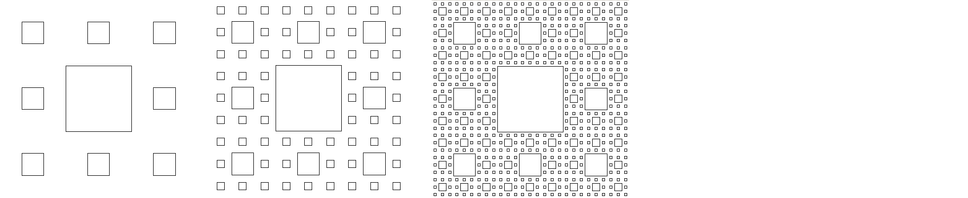
Chapter 5 Exercises

Add the following methods to the binary tree class of Section 5.2.
1. count(x) — returns how many things in the tree are equal to x. When checking if things are equal to x, use .equals instead of ==.
2. isEqual(t) — returns true if the tree is equal to the tree t. Two trees are considered equal if they have the same values in the exact same tree structure.
3. get(location) — Takes a location string of L's and R's, similar to the one used by the add method, and returns the item at that location in the tree. You can assume that the caller's string is a valid location in the tree.
4. isUnbalanced() — returns true if there is some node for which either its left subtree or right subtree is more than one level deeper than the other
5. leaves() — returns a list containing the data in all the leaves of the tree
6. level(location) — returns the level of the node specified by the string location, assuming the root is at level 0, its children are at level 1, their children are at level 2, etc.
7. locationOf(x) — Takes an integer x and returns the location of it in the tree. If x is at the root, return "Root". If x is not in the tree, return "Not found". Otherwise, return the location as a string of L's and R's that leads to its location. If the item occurs in multiple places below the root, your program can return whichever one of those locations it wants.
8. numberOfDescendants(location) — returns the number of descendants of the node whose location is given by the string location. Descendants of a node include its children, its childrens' children, etc.
9. numberOfFullNodes() — Recall that nodes in a binary tree have 0, 1, or 2 children. This method returns how many nodes in the tree have exactly two children (only children, not grandchildren or other descendants).
10. parenthesizedRepresentation() — returns a string containing a parenthesized representation of the tree. The basic structure of the representation at a node is
  (data value, representation of left subtree, representation of right subtree). If a node doesn't have a left or a right subtree, the representation for the missing subtree is *. As an example, the tree below has the following representation:
```
   (3,(5,(9,*,*),(1,*,(4,*,*))),(6,(2,*,*),*))
```
11. printLevel(k) — prints all of the elements at level k
12. set(location, value) changes the data value at the node specified by the string location to the given new value.
Our binary tree class works with generic types. Make the class less general so that it only works with integer data. Then add the following methods to the class:
1. max() — Returns the largest integer stored in the tree.
2. numNegatives() — Returns how many negative entries are in the tree
3. numNegativeLeaves() — Returns how many leaves in the tree have negative values
4. sum() — Returns the sum of all the integers stored in the tree.
5. sumByDepth — returns the sum of the elements in the tree, weighted by depth. The root is weighted by 1, each of its children is weighted by 2, each of their children is weighted by 3, etc.
Rewrite the size method using an iterative, instead of recursive, algorithm.
Rewrite the binary tree class to represent a general tree where each node can have an arbitrary number of children. To do this, use a list of nodes in place of the left and right variables.
Write a binary tree class that uses an dynamic array instead of a linked structure. Use the following technique: The root is stored at index 0. Its children are stored at indices 1 and 2. The children of the root's left child are stored at indices 3 and 4, and its right children are stored at indices 5 and 6. In general, if the index of a node is i, then its left and right children are stored at indices 2i+1 and 2i+2, respectively. The class should have three methods:
- setRoot(value) — sets the value of the root node
- set(location, value) — takes a string, location, of L's and R's representing the location, and sets the corresponding node to value
- toString() — returns a string representing an in-order traversal of the tree

Chapter 6 Exercises

The following items are added to a binary search tree (BST) in the order given. Sketch what the tree will look like after all the items are added. 15, 25, 6, 2, 4, 9, 23, 8, 10
Use the BST below for this problem. Sketch what the tree will look like after deleting the following elements: (a) Delete 35 (b) Delete 20 (after 35 has already been deleted)
This is not a BST. Indicate precisely where the BST property is broken.
1. What are defining properties of a BST?
2. In deleting an item with two children, we replace it with an item from exactly where in the tree?
3. Explain why using that item preserves the defining properties of a BST. In particular, once it's in its new location, why will everything to the left of it be less than or equal to it and everything to the right of it be greater than it?
4. Besides the answer given in part (b), there is one other item that we could use. What is it?
If the binary search tree is well-balanced, what are the big O running times of adding and deleting?
If elements are added to a binary search tree in numerical order (and no effort is made to rebalance the tree), what are the big O running times of adding and deleting items?
This exercise involves adding some methods to the BST class. Your methods must make use of the order property of binary search trees. In other words, they should work with binary search trees, but not on an arbitrary binary tree. Except for the last problem, these methods should not have to look at every item in the tree. Binary search trees are ordered to make searching faster than with arbitrary trees and this problem is about taking advantage of that ordering.
1. get(k) — returns the kth smallest item in the BST
2. max() — returns the maximum item in the BST
3. min() — returns the minimum item in the BST
4. midrange() — returns the midrange of the items in the BST. The midrange of a collection of values is the average of the smallest and largest values. For instance, the midrange of 4, 5, 8, 10 is (4+10)/2=7 . If the BST has only one value in it, use that value as the midrange, and if the BST is empty, throw a runtime exception.
5. numberLess(n) — returns the number of elements in the tree whose values are less than n. Do not use the toArrayList method from this problem.
6. successor(x) — returns the next largest item in the tree greater than or equal to x. Throw an exception if there is no such item.
7. toList() — returns an ArrayList containing the elements of the tree in increasing order. Use the ordering property of BSTs, rather than calling a sort method, to make sure the elements are increasing order.
Write a method called BSTSort(List<Integer> list) in a separate file (i.e. not in the BinarySearchTree class file). It should take a list of integers and return a new list of integers that is a sorted version of the original. Your method should use the following algorithm to do the sorting: Add the elements one-by-one from the list into a BST and then call the toList method (given in the previous problem).
It would be nice if Java had a special class for ordered pairs (things like (2,3) or (5,1) that you might remember from algebra). Java unfortunately doesn't have such a class, but we can create one. Create a class called OrderedPair with the following specifications.
1. There are two private integer variables x and y.
2. There is a constructor that sets the two values to values supplied by the caller.
3. There are getters (but no setters) for each variable.
4. There is a toString method that returns a string of the form "(x,y)", where x and y are the actual values of the x and y variables.
5. There are equals and hashCode methods. These methods are necessary for the class to play nice with other things in Java. Do not write the code for these by hand. Instead, use your IDE to generate these for you. Eclipse has an option for this under the Source menu.
6. The class should implement the Comparable interface and have a compareTo method that compares two OrderedPair objects p1 and p2 according to this rule:
  - p1 and p2 are equal if their x and y variables are both equal.
  - p1 is smaller than p2 provided p1.x < p2.x or if p1.x equals p2.x and p1.y < p2.y.
  - Otherwise p2 is larger than p1.
  For instance, OrderedPair(2,8) is smaller than OrderedPair(3,5) and OrderedPair(2,9).
7. In the main method, create a list of 100 OrderedPair objects, each with randomly generated x and y values from 1 to 10.
8. Use Collections.sort to sort the list, and then print out the list.
9. Use the ArrayList contains method to print out whether or not (1,1) is in the list.

Chapter 7 Exercises

The tree below is not a heap. There are two particular reasons why it is not a heap, one having to do with the structure of the tree and the other having to do with the values. Give both reasons and indicate precisely where in the tree each occurs.
Elements are added to a heap in the order given below. Draw the heap at each individual step.

Step 1: 9 is added Step 2: 16 is added
Step 3: 3 is added Step 4: 2 is added
Step 5: 10 is added Step 6: 4 is added
Show what the heap below will look like after a heap pop() operation is performed.
Recall that heaps are implemented using lists. What would the list be for the original heap shown in problem 3?
Add the following methods to the Heap class:
1. delete(x) — Deletes an arbitrary element x from the heap. One way to do this is to do a linear search through the list representing the heap until you find the element and then delete it in more or less the same way to how the pop method removes the min. If there are multiple copies of x, your method doesn't have to delete all of them.
2. numberOfPCCMatches() — returns how many nodes in the heap have the same values as both of their children.
Create a class called MaxHeap that is like the Heap class except that it implements a max heap, where a parent's value is always greater than or equal to both of its children.
Create a class called MaxHeap2 that has the same methods as the Heap class, but uses Java's PriorityQueue class under the hood to implement the methods. Assume that the data in the heap is all integers. [Hint: mathematically, if x>y then -x<-y.]
Create a class called GHeap that is a generic version of the Heap class that works with any data type that implements the Comparable interface. Make sure the class has the same methods as the Heap class.
Write a static method, heapFunction(list) that takes a list of integers and adds them all one-by-one to a heap (using Java's PriorityQueue). Then it removes them all one-by-one from the heap, putting them all back into the caller's list, replacing the values that are currently there. It's a void method; it modifies the caller's list but returns nothing. In the main method create a list of 100 random integers from 50 to 200, print it, call the method on that list, and print the list again. If your method is working, the second time you print the list, the values will be in order.
Create a method representsHeap(list). This is a static method in a class separate from the Heap class that takes a list of integers as a parameter and returns true or false depending on if the list could represent a heap. To write this method, you have to verify that in the list each parent's value is always less than or equal to its childrens' values. Recall that the children of the node at list index p are located at indices 2p+1 and 2p+2. [Note: be careful near the end of the list that you don't get an index out of bounds error.]
One nice application of heaps is for sorting really huge data sets, like data from a file several gigabytes in size, where it would be impossible to fit all of the data into RAM at once. Suppose we have a huge file consisting of integers, and we need to know the 10 largest integers from the file. Here is an algorithm to find them: Start by reading the first 10,000 items from the file. Add them all into a heap. Pop the first 10 things off of the heap and add them to a new heap. Then add the next 9990 items from the file onto that heap. Pop the first 10 things off of this heap onto a new heap and add the next 9990 items from the file onto that heap. Keep repeating this process until you've gone through all the data in the file. Popping the first 10 things off of the last heap gives the ultimate solution. Implement this algorithm in a function called largest10. The function should take a string argument representing a filename and return a list of the 10 largest integers from that file. Assume the file contains one integer per line.

Chapter 8 Exercises

Consider the hash function h(x) = 3x mod 5 that operates on integers. Suppose we use this hash function with a hashing implementation of a set, using the chaining approach we covered in class.
1. How many buckets are there?
2. Suppose we add the elements 7, 16, 2, 9, 6. Sketch what the buckets must look like.
3. Give an example of a collision from this hash function.
1. If we use a good hash function, the buckets will all only have at most a few elements each. This means that add, remove and contains will all have what big O running time?
2. If we use a bad hash function and most of the elements end up in the same couple of buckets, what will the (worst-case) big O running time be for the three methods in part (a)?
1. Write a static method called numUnique(list) that takes a list as a parameter and returns how many unique elements are in the list. For instance, if the list is [1,2,3,2,7,10,7], the method should return 5 because there are 5 unique items in the list, namely 1, 2, 3, 7, and 10. You must do this problem using sets (it's actually only 1 or 2 lines that way). Your method should work with any data type, not just integers. To do that, the method signature should be public static <T> int numUnique(List<T> list).
2. Test your method by using a loop to create a list of 50 random lowercase letters and calling the method on that list. [Note: you must create the list with a loop, not using 50 separate calls to the add method or using Collections.addAll().]
1. Write a static method called symmetricDifference(list1, list2) returns a set of all the items that are in list1 or list2 but not both. For instance, if list1 is [1,2,4,1,5] and list2 is [2,3,4], the method would return {1,3,5}. Make sure it works with any type of list, not just integer lists.
2. Test your method by creating two lists of 100,000 elements that contain random numbers from 1 to 100,000. Call the symmetricDifference method on these two sets and print out the size of the set it returns. Your answer will come out around 46,500. [Note: Your method should return its answer instantly. If it's not then something is wrong. The way to fix that is to make sure to convert list2 into a set in the method.]
The files pride_and_prejudice.txt and war_and_peace.txt contain the entire texts of two famous novels. For this problem, you will be finding all the words that are in War and Peace but not in Pride and Prejudice.
1. Do this by creating a set of all the words in Pride and Prejudice and another set of all the words in War and Peace and seeing what is in the latter that is not in the former. Be sure to remove all the punctuation and convert the text to lowercase.
2. Repeat the above but use a list instead of a set.
3. How long did the first program take to find all the words? How long did the second one take?
4. How does your answer in part (c) relate to the big O of looking through a set and a list/array for something?
This exercise is about a simplification of the HSet class. In place of a list of buckets, it uses a list of booleans. To add an item to the set, we compute its hash and store a value of true in the corresponding index of the boolean list. Note that this means that this data structure doesn't actually store the value. It's just a record of whether or not a specific value has ever been added to the data structure. And because of hash collisions, it might not even accurately record that. However, it is super efficient and will usually return the right answer, just not always. In real-life problems, sometimes getting an answer that is usually but not always right is okay, especially if the answer comes quickly.
Call this class PseudoSet. It will have an instance variable of type List<Boolean> that holds the “data” of the set. Give it the following methods:
1. PseudoSet() — a constructor that creates an empty set.
2. h(x) — the same hash function we used in the HSet class.
3. add(x) — adds x to the set by computing its hash value and storing true at the corresponding index of the boolean list.
4. contains(x) — returns whether or not the set likely contains the value x by computing the hash value of x and looking at the corresponding entry in the boolean list.
A bitset is a way of implementing a set where the set's data is stored in an array of booleans such that index i in the array is set to true if i is in the set and false otherwise. For instance, the set {0, 1, 4, 6} is represented by the following array:
```
    [true, true, false, false, true, false, true]
    
```
The indices 0, 1, 4, and 6 are true, and the others are false. Write a BitSet class that works for sets of integers that contains the following methods:
1. [] BitSet(n) — a constructor that creates an empty set. The parameter n specifies the largest element the set will be able to hold. This parameter is thus the size of the boolean array.
2. [] BitSet(list) — a constructor that is given an ArrayList of integers and builds a set from it
3. [] toString() — returns a string containing the contents of the set bracketed by curly braces with individual elements separated by commas and spaces. For example: {0, 1, 4, 6} is how the set above would be returned.
4. [] toList() — returns an ArrayList of integers containing the elements of the set
5. [] contains(x) — returns true or false depending on whether the set contains the element x
6. [] add(x) — inserts x into the set
7. [] remove(x) — removes x from the set
8. [] size() — returns the number of elements in the set
9. [] isEmpty() — returns true if the set is empty and false otherwise
10. [] getMax() — returns the largest element that the set is able to hold
11. [] union(s1, s2) — a static method that returns the union of sets s1 and s2. [Be careful because the sets may have different sizes.]
12. [] intersection(s1, s2) — a static method that returns the intersection of sets s1 and s2. [Be careful because the sets may have different sizes.]
13. [] difference(s1, s2) — a static method that returns the intersection of sets s1 and s2. [Be careful because the sets may have different sizes.]
14. [] isSubset(s1, s2) — a static method that returns whether or not s1 is a subset of s2.
Implement a set using a binary search tree. Provide add, remove, contains, and union methods.

Chapter 9 Exercises

What does the function below accomplish? Assume c is a character in s.

public static int f(String s, char c) {
    Map<Character, Integer> map = new LinkedHashMap<Character, Integer>();
    for (int i=0; i<s.length(); i++) {
        if (map.containsKey(s.charAt(i)))
            map.put(s.charAt(i), map.get(s.charAt(i))+1);
        else
            map.put(s.charAt(i), 1);
    }
    return map.get(c);
}

Write a few lines of code that creates the map {"a":4, "b":2, "c":3} and then uses that map to create a string consisting of the keys of that map repeated a number of times equal to their values. For this map, it would be "aaaabbccc".
Write a function called validDate that takes a string in the format of a month name followed by a day number (like "November 29"). It should return a boolean indicating whether the date is real. A date is considered real if its month name is spelled correctly and its day number is in the range from 1 to the number of days in the month. For instance, January 0, February 30, and Febray 25 are not real dates. Do this problem by creating a map whose keys are month names and whose values are the number of days in each month (29 for February, 30 for April, June, September, and November, 31 otherwise).
The file elements.txt contains periodic table data. Write a program that reads the file and creates a map whose keys are the element symbols (H, He, Li, etc.) and whose values are the corresponding names of those elements: (Hydrogen, Helium, Lithium, etc.) Then ask the user to enter an abbreviation and print out its name. If the abbreviation is not a valid element abbreviation, print out a message saying so.
Write a method called sameCharFreq(s, t) that takes two strings and returns whether they contain the same characters with the same frequencies, though possibly in different orders. For instance, "AABCCC" and "CCCABA" both contain two As, a B, and three Cs, so the method would return true for those strings. It would return false for the strings "AAABC" and "ABC" since the frequencies don't match up. Your method should use a map.
This problem will give you a tool for cheating at crossword puzzles. Create a function called crosswordCheat(s) that takes a string s that consists of the letters they know from the word, with asterisks as placeholders for the letters they don't know. Then print a list of all the words that could work. For instance, if s is w**er, the program should return a list containing water, wafer, wider, etc.
Please do the problem using a map as follows: Create a map map1 from s so that its keys are the indices of the non-asterisk characters and its values are the characters themselves. Then loop through the words in a wordlist. If the word has a different length than s, then move on to the next word. Otherwise, create a similar map, map2 for the word, and compare the two maps. If map1 has any keys that are not in map2 or if the value associated with any key of map1 is different from its value in map2, then the word won't work. Otherwise, it will, and print it out.
Suppose we are given a word, and we want find all the words that can be formed from its letters. For instance, given water, we can form the words we, wear, are, tea, etc.
One solution is, for a given word, form a map whose keys are the characters of the word and whose values are the number of times the character appears in the word. For instance, the map corresponding to java would be {a:2, j:1, v:1}. A word w can be made from the letters of another word W if each key in the map of w also occurs in the map of W and the corresponding values for the letters of w are less than or equal to the values for the letters of W.
Using this approach, write a method called wordsFrom that takes a string and returns a list of all the English words (from a wordlist) that can be made from that string.
One use for maps is for implementing sparse integer lists. A sparse integer list is one where most of the entries are 0, and only a few are nonzero. We can save a lot of space by using a map whose keys are the indices of nonzero entries and whose values are the corresponding entries. Create a class called SparseList that uses this approach. The class should have get, set, and contains methods. In this exercise, you are creating what is basically an implementation of a list that uses maps. What is special about it is that the map only stores the indices of nonzero values.
The file scores.txt contains the results of every 2009-10 NCAA Division I basketball game (from http://kenpom.com). Each line of that file looks like below: 11/09/2009 AlcornSt. 60 OhioSt. 100
Write a program that finds all the teams with winning records (more wins than losses) who were collectively (over the course of the season) outscored by their opponents. To solve the problem, use maps wins, losses, pointsFor, and pointsAgainst whose keys are the teams.
The substitution cipher encodes a word by replacing every letter of a word with a different letter. For instance every a might be replaced with an e, every b might be replaced with an a, etc. Write a program that asks the user to enter two strings. Then determine if the second string could be an encoded version of the first one with a substitution cipher. For instance, CXYZ is not an encoded version of BOOK because O got mapped to two separate letters. Also, CXXK is not an encoded version of BOOK, because K got mapped to itself. On the other hand, CXXZ would be an encoding of BOOK.
Suppose you are give a file courses.txt, where each line of that file contains a name and the CS courses that person has taken. Read this info into a map whose keys are the names and whose values are lists of courses. Then create a static method called getStudents(map, course) that takes the map and a course number and uses the map to return a list of all the students who have taken that course.
The file war_and_peace.txt contains the complete text of Tolstoy's War and Peace. Convert it all to lowercase and create a map that whose keys are the lowercase letters a through z and whose values are what percentage (as a double) of the total that letter comprises, each rounded to 1 decimal place. Your final map should start with the exact entries below (in alphabetical order) when printed out:
```
    {a=8.1, b=1.4, c=2.4, d=4.7, e=12.5, ...
    
```
That is, 8.1% of the letters are a's, 1.4% are b's, etc. Hint: This line can be used to read the entire contents of a file into a string in one fell swoop:
```
    String text = new String(Files.readAllBytes(Paths.get("war_and_peace.txt")));
    
```

Below are the notes used in music:

C C# D D# E F F# G G# A A# B

The notes for the C major chord are C, E, G. A mathematical way to get his is that E is 4 steps past C and G is 7 steps past C. This works for any base. For example, the notes for D major are D, F#, A. We can represent the major chord steps as a list with two elements: [4, 7]. The corresponding lists for some other chord types are shown below:

Minor	`[3,7]`	Dominant seventh	`[4,7,10]`
Augmented fifth	`[4,8]`	Minor seventh	`[3,7,10]`
Minor fifth	`[4,6]`	Major seventh	`[4,7,11]`
Major sixth	`[4,7,9]`	Diminished seventh	`[3,6,10]`
Minor sixth	`[3,7,9]`

Write a program that asks the user for the key and the chord type and prints out the notes of the chord. Use a map whose keys are the (musical) keys and whose values are the lists of steps.

Chapter 10 exercises

Give the adjacency list representation of the graph below.
For the graphs below, we are starting at vertex a. Indicate the order in which both breadth-first search and depth-first search visit the vertices.
Mathematicians are interested in what is called their Erdős number. Paul Erdős was a prolific mathematician who had hundreds of collaborators. Anyone who coauthored a paper with Erdős himself has an Erdős number of 1. Anyone else who coauthored a paper with someone who coauthored a paper with Erdős has an Erdős number of 2. Erdős number 3, 4, etc. are defined analogously. We would like to write a program where we enter a mathematician's name and the output is their Erdős number. Find a way to represent the problem with a graph. Say what the vertices and edges are and how the problem could be solved.
Here is a puzzle that is at least 1200 years old: A traveler has to get a wolf, a goat, and a cabbage across a river. The problem is that the wolf can't be left alone with the goat, the goat can't be left alone with the cabbage, and the boat can only hold the traveler and a single animal/cabbage at once. How can the traveler get all three items safely across the river?
One approach is to make the vertices be the possible states of the puzzle as strings. You can use a string like "WC|GP" to mean that the wolf and cabbage are on the left side of the river and the goat and person are on the right side of the river. You would only need to make vertices for legal states of the puzzle. Edges go from each state to all the states it is possible to get to from that state with a single crossing.
1. Sketch the graph and use it to find two solutions to the puzzle.
2. Using the Graph class, add all the vertices and edges for this graph and then use BFS to find a solution.
Shown below are two states of a slider puzzle, also known as the 15 puzzle. The goal of the puzzle is to slide around the tiles using the one blank spot to get from a mixed-up state like on the left to the solve state on the right. If you're not sure how they work, google “15 puzzle”.
Describe how to solve this problem with graph theory as below:
1. Describe what to make the vertices and what to make the edges.
2. For the particular case of the state of the puzzle above on the left, give exactly what the vertices and edges associated with that state would be.
3. What algorithm would you use to find a sequence of moves that take the puzzle from the state on the left to the state on the right?
A floodfill is where you have a two-dimensional region and you fill part of it with a certain value until you reach boundaries. Those boundaries can be the edge of the region or other values in the region. This is a common feature in many drawing programs. It is also useful in certain games, like Minesweeper. As an example, a region (two-dimensional array of characters) is shown below on the left. We want to floodfill parts of the region by replacing dashes with @ symbols. The result of floodfilling starting at index (0,0) is shown in the middle. There we start by setting the dash at (0,0) to @. From there we continue searching up, down, left, and right until we reach the end of the array or an asterisk character. On the right below is the result of a floodfill starting at index (1,3).
```
- - * - * -       @ @ * - * -       - - * @ * -
- * - - * *       @ * - - * *       - - * @ * -
* * * - - *       * * * - - *       * * * @ @ *
- * - - * *       - * - - * *       - * @ @ * *
- * * - - -       - * * - - -       - * * @ @ @
```
Write a function called floodfill(char[][] a, int r, int c) that takes a two-dimensional array of characters and a location (r,c) and performs a floodfill replacing dashes with @ characters, starting at location (r,c). Your function should modify the caller's array. Instead of creating a graph, do this by modifying the BFS or DFS code to work with an array.
In the game Boggle, letters are arranged in a 5× 5 grid. The goal is to try to find words in the grid. You form words by picking a starting letter and following a path from cell to cell. You can move horizontally, vertically, or diagonally, and this can be done backwards or forwards. For example, in the board below, if we start at the B near the bottom right, we can form the word BYTES by moving right, then up, then left, and then diagonally left and down.
```
B D N V M
S T M C B
I M E N A
S P K E T
T L S B Y
```
Write a function called boggleWords(a) that finds all the words of 3 to 8 letters that can be formed from a Boggle board. Assume the board is given as an two-dimensional array of characters. Do this by modifying the code for DFS.
Consider the puzzle problem below. Find a way to represent it as a graph, program that implementation, and run breadth-first search on it to find a solution.

Five professors and their five dogs were having a lot of fun camping. Each professor owned one of the dogs. While they were all on a hike, they came to a river they had to cross. There was a small motorboat alongside the river. They determined that the boat was only large enough to hold three living things—either dogs or professors. Unfortunately, the dogs were a little temperamental, and they really didn't like the professors. Each dog was comfortable with its owner and no other professor. Each dog could not be left with the professors unless the dog's owner was present—not even momentarily! Dogs could be left with other dogs, however. The crossing would have been impossible except Professor A's dog, which was very smart, knew how to operate the boat. None of the other dogs were that smart, however. How was the crossing arranged, and how many trips did it take?
Add the following methods to the Graph class.
1. size() — returns the number of vertices in the graph.
2. numberOfEdges() — returns how many edges are in the graph.
3. isEmpty() — returns whether or not there are any vertices in the graph.
4. degree(v) — returns how many neighbors vertex v has.
5. contains(v) — returns whether or not v is a vertex in the graph.
6. containsEdge(u,v) — returns whether or not there is an edge between u and v.
7. remove(v) — removes vertex v from the graph.
8. removeEdge(u,v) — removes the edge between u and v from the graph.
9. toString() — returns a string representation of the graph, with each line consisting of a vertex name, followed by a colon, followed by the vertex's neighbors, with a space between each neighbor. For instance, if the graph consists of vertices a, b, c, d, and e with edges ab, ac, and cd, the string should look like the following:
```
    a : b c
    b : a
    c : b d
    d : c
    e :
    
```
10. distance(u,v) — returns the distance between two vertices. The distance is the length of the shortest path between the vertices.
11. isConnectedTo(u, v) — returns true if it is possible to get from vertex u to vertex v by following edges.
12. isConnected() — returns true if the graph is connected and false otherwise. A graph is connected if it is possible to get from any vertex to any other vertex.
13. findComponent(v) — returns a list of all the vertices that can be reached from vertex v
14. components(v) — returns a list of all the components of a graph. A component in a graph is a collection of vertices and edges in the graph such that it is possible to get from any vertex to any other vertex in the component.
15. isCutVertex(v) — returns true if v is a cut vertex, a vertex whose deletion disconnects the graph.
16. isHamiltonianCycle(a) — returns true if the list of vertices a represent a Hamiltonian cycle. A Hamiltonian cycle is a cycle that includes every vertex.
17. isValidColoring(m) — returns true if the map m represents a valid coloring of the graph and false otherwise. A coloring of a graph is an assignment of colors to the vertices of the graph such that adjacent vertices are not given the same color. The argument m is a map whose keys are the vertices of the graph and whose values are the colors (integers) assigned to the vertices. Usually positive integers are used for the color names.
18. findValidColoring() — returns a map like in the previous problem that represents a valid coloring of the graph. Create the map using the following greedy algorithm: Loop through the vertices in any order, assign each vertex the smallest color (starting with the number 1) that has not already been assign to one of its neighbors.
19. isEulerian() — returns true if the graph is Eulerian and false otherwise. A graph is Eulerian if one can traverse the graph using every edge exactly once and end up back at the starting vertex. A nice theorem says that a graph is Eulerian if and only if every vertex has even degree.
20. inducedSubgraph(list) — given a list of vertices, returns a new graph object which consists of the vertices in the list and all the edges in the original graph between those vertices.
In a file separate from the Graph class, create the following methods:
1. addAll(G, s) — Assuming G is a graph whose vertices are strings and s is a string with vertex names separated by spaces, this method adds vertices to G for each vertex name in s. For instance, if s = "a b c d", this method will add vertices named a, b, c, and d to the graph. Vertex names may be more than one character long.
2. addEdges(G, s) — Assuming G is a graph whose vertices are strings and s is a string of edges separated by spaces, this method adds edges to g for each edge name in s. Each edge is in the form endpoint1-endpoint2. For instance, if s = "a-b a-c b-c", this method will add edges from a to b, from a to c, and from b to c. Vertex names may be more than one character long.
Add methods called indegree and outdegree to the Digraph class. The indegree of a vertex is the number of edges directed into it, and the outdegree of a vertex is the number of edges directed out from it.
Modify the depth-first search and breadth-first search methods so that instead of a single goal vertex as a parameter, they receive a list of goal vertices as a parameter. The search is successful if any of the vertices in the list are found.
Write a recursive version of the depth first search algorithm.
Modify the depth-first search algorithm to create a function hasCycle(G) that determines if the graph G has a cycle. [Hint: if depth-first search encounters a vertex that it has already seen, that indicates that there is a cycle in the graph. Just be careful that that vertex doesn't happen to be the parent of the vertex currently being checked.]
Modify the depth-first search algorithm to create a function isBipartite(G) that determines if the graph G is bipartite. A graph is bipartite if its vertices can be partitioned into two sets such that the only edges in the graph are between the two sets, with no edges within either set. One way to approach this problem is to label each vertex as you visit it with a 0 or 1. Labels should alternate so that all the neighbors of a vertex v should have the opposite label of what v has. If there is ever a conflict, where a vertex is already labeled and this rule would try to assign it a different label, then the graph is not bipartite.

Chapter 11 exercises

Consider the array [T, S, Y, F, R, B].
1. Show how Selection Sort works on the array by showing exactly what elements are swapped and when.
2. Repeat part (a) for Bubble Sort.
3. Repeat part (a) for Insertion Sort.
Consider the array [M, D, W, N, P, B, C, Y].
1. Mergesort will initially break this array into two pieces. What are those two pieces?
2. Quicksort will initially break this array into two pieces. What are those two pieces if the first element is used as the pivot?
Suppose that mergesort has broken an array into two parts and sorted those two parts into [C, R, S, V] and [D, M, T, Y, Z]. Show each step of the merge process that merges those two parts into one big array.
Suppose that quicksort has broken an array into two parts and sorted those parts into [B, D, F, R], and [T, W, Z]. If the pivot is S, describe how quicksort combines everything back into one big array.
Show how the in-place quicksort partition operation works on the list below, using the first element of the list as a pivot. Please show your work clearly, indicating how the indices move through the list and when swaps occur.
[M, N, W, T, R, U, F, K, Y, E, B, A, V, O, H, S, P]
You are showing just the partition process in this problem, not the recursive part of quicksort.
Fill in the missing entries in the table of big O running times below.
Algorithm Worst Case Best Case Average Case
Insertion sort
Mergesort O(n log n)
Quicksort O(n log n)
1. Give an example of a array of 10 items for which quicksort will run in O(n²) time if it always uses the first item as a pivot.
2. If the pivot is changed to always pick the middle element, will the running time for your array be O(n²) or O(n log n)?
Explain how quicksort can degenerate to O(n²) if the array consists of just a few values repeated quite a bit, like an array of 1000 ones, 1500 twos, and 80 threes, all jumbled up.
At the end of the part of Section 11.5 on Bubble Sort was a suggestion for improving Bubble Sort by checking to see if any swaps were made on a pass through the array. If no swaps are made, then the array must be sorted and the algorithm can be stopped. Implement this.
In Section 11.7, we showed how to write the selection sort variant to work with a generic list. Rewrite the Quicksort method in the same way.
Exercise 9 of Section 12.6 asked you to create a class called OrderedPair that represents an ordered pair (x,y). Create a list of pairs and sort the pairs by their x coordinates. Then perform a sort that sorts them first by their x coordinates and second by their y coordinates.
Write a method that takes a string of lowercase letters and creates a map of how many times each letter appears. Using that map, do the following:
1. Print out the letters and their frequencies, ordered alphabetically.
2. Print out the letters and their frequencies, ordered from most to least frequent.
3. Print out the letters and their frequencies, ordered from least to most frequent.
Implement the following sorting algorithms to sort integer arrays.
1. Treesort — This works just like Heapsort except it uses a BST in place of a heap. Do this using the BST class from Chapter 7. In particular, you will want to add a method to that class called inOrderList that returns a list of the items in the BST from an in order traversal.
2. Cocktail sort — This is a relative of bubble sort. Assume the n elements are in indices 0, 1, … n-1. Start by comparing elements 0 and 1, then elements 1 and 2, and so on down to the end of the array, swapping each time if the elements are out of order. When we're done, the largest element will be in place at the end of the array. Now go backwards. Start at the second to last element (index n-2) and compare it with the one before it (index n-3). Then compare the elements at n-3 and n-4, the elements at n-4 and n-5, etc. down to the front of the list. After this, the smallest element will be in place at the front of the array. Now proceed forward again, starting by comparing elements 2 and 3, then 3 and 4, etc., down to n-3 and n-2. After this the second to last element will be correct. Then go backwards again, then forwards, then backwards, each time stopping one position short of the previous stopping place, until there is nowhere left to move.
3. Hash table counting sort — This is like counting sort, except instead of using an array of counts, it uses HashMap of counts.
4. Introsort — This is a combination of Quicksort and Heapsort. Introsort uses the Quicksort algorithm to sort the array until some maximum recursion depth is reached (say 16 levels deep), at which point it switches to Heapsort to finish the sorting.
5. Odd/even sort — Implement the following sorting algorithm: Start by comparing the elements at indices 1 and 2 and swapping if they are out of order. Then compare the elements at indices 3 and 4, 5 and 6, 7 and 8, etc., swapping whenever necessary. This is called the “odd” part of the algorithm. Then compare the elements at indices 0 and 1, 2 and 3, 4 and 5, 6 and 7, etc., swapping whenever necessary. This is called the “even” part of the algorithm. What you do is do the odd part, then the even part, then the odd part, then the even part, etc. repeating this process until the list is sorted. One way to tell if the list is sorted is that once you do an odd part followed by an even part, and no swaps are made in either part, then the list is sorted.
6. Comb sort — Comb sort is a modification of bubble sort that instead of comparing adjacent elements, instead compares elements that are a certain gap apart. There are several passes with the gap size gradually decreasing. Essentially, comb sort is to bubble sort as shell sort is to insertion sort. The starts at size n/1.3 and by a factor of 1.3 until the gap size is 1, which is what is used for the final pass. On each pass, an algorithm analogous to bubble sort is performed except that instead of comparing adjacent elements, we compare elements that are one gap apart.
7. Bucket sort — This sort puts the data into different “buckets,” sorts the buckets individually, and then puts the buckets back together. Write a simple version of this algorithm that assumes the data consists of integers from 0 to 999999, sorts it into buckets of size 100 (0-99, 100-199, 200-299), and uses insertion sort on each bucket.
8. Radix sort — This sort works by sorting integers based on their ones digit, then on their tens digit, etc. A simple version of this can be implemented as follows: Put the elements of the array into one of ten buckets, based off their ones digit. Put the elements back into the array by starting with all the elements in the 0 bucket, followed by all the elements in the 1 bucket, etc. Then put the elements back into buckets by their tens digit and fill the array back up in order from the buckets. Repeat this process until there are no more digits to work with.
9. Permutation sort — This is a really bad sort, but it is a good exercise to try to implement it. It works by looking at all the permutations of the elements until it finds the one where all the elements are in sorted order. One way to implement it is to generate all the permutations of the indices 0, 1, …, n-1 (see Section 4.3), create a new array with the elements in the order specified by the permutation, and check to see if the elements of the new array are in order.
10. Bogosort — This is another really bad sort—it runs in worse than O(n!) time. The way it works is it randomly shuffles the elements of the array until they are in order. One way to implement this is to put the elements of the array into a list and use Collections.shuffle.

`n`	`onesAndTwos(n)`
1	`["1"]`
2	`["11", "2"]`
3	`["111", "21", "12"]`
4	`["1111", "112", "121", "211", "22"]`

Step 1: 9 is added	Step 2: 16 is added
Step 3: 3 is added	Step 4: 2 is added
Step 5: 10 is added	Step 6: 4 is added

Algorithm	Worst Case	Best Case	Average Case
Insertion sort
Mergesort		O(n log n)
Quicksort		O(n log n)

Links

Preface

Running times of algorithms

Introduction

Estimating the running times of algorithms

Common running times

Some notes about big O notation

Logarithms and Binary Search

Lists

Dynamic arrays

Implementing a dynamic array

Adding elements

Displaying the contents of the dynamic array

More methods

Running times

Linked lists

Implementing a linked list

Working with linked lists

Basics

Looping

Using pictures

Edge cases

Null pointer exceptions

A couple of trickier examples

More about linked lists

Comparing dynamic arrays and linked lists

Doubly- and circularly-linked lists

Making the linked list class generic

Lists in the Java Collections Framework

List methods

Methods of java.util.Collections

A couple of examples

Stacks and Queues

Introduction

Stacks

Queues

Deques

Implementing a stack

Implementing a queue

Stacks, queues, and deques in the Collections Framework

Applications

Recursion

Introduction

Basic recursion examples

Length of a string

Sum of a list

Fibonacci numbers

A contains method

Smallest element of a list

Testing for palindromes

Repeating a string

A range function

A replaceAll method

Determine if all elements of a list are 0

Power function

Finding the index of a character

Finding repeats

Minimum of a list (again)

Summing a list (again)

Minimum of a list (one more time)

More sophisticated uses of recursion

Printing the contents of a directory

Factoring numbers

Permutations

Combinations

The Sierpinski triangle

Towers of Hanoi

Working with recursion

Stack overflow errors

Using parameters

Tail recursion

Summary

Binary Trees

Introduction

Implementing a binary tree

Binary trees and recursion

A size method

A contains method

A height method

A method to count leaves

`List` methods

Methods of `java.util.Collections`

Java's `Comparable` interface

A `toString` method