A Simple Introduction to Graph Theory

Here is a pdf version of the book.

Preface

These are notes I wrote up for my graph theory class in 2016. They contain most of the topics typically found in a graph theory course. There are proofs of a lot of the results, but not of everything. I've designed these notes for students that don't have a lot of previous experience in math, so I spend some time explaining certain things in more detail than is typical. My writing style is also pretty informal. There are a number of exercises at the end.

If you see anything wrong (including typos), please send me a note at heinold@msmary.edu.

Basics

What is a graph?

Graphs are networks of points and lines, like the ones shown below.

They are useful in modeling all sorts of real world things, as we will see, as well as being interesting in their own right. While the figure above hopefully gives us a reasonably good idea of what a graph is, it is good to give a formal definition to resolve any ambiguities.

A graph is a pair (V,E), where V is a set of objects called vertices and E is a set of two element subsets of V called edges.

So a graph is defined purely in terms of what its vertices (points) are, and which vertices are connected to which other vertices. Each edge (line) is defined by its two endpoints.

It doesn't matter how you draw the graph; all that matters is what is connected to what.

For instance, shown below are several ways of drawing the same graph. Notice that all three have the same structure of a string of five vertices connected in a row.

For the second and third examples above, we could imagine moving vertices around in order to “straighten out” the graph to look like the first example. Notice in the third example that edges are allowed to cross over each other. In fact, some graphs can't be drawn without some edges crossing. Edges are also allowed to curve. Remember that we are only concerned with which vertices are connected to which other ones. We don't care exactly how the edges are drawn.

In fact, we don't even have to draw a graph at all. The graph above can be simply defined by saying its vertices are the set V = {a,b,c,d,e} and its edges are the set E = {ab, bc, cd, de}. However, we will usually draw our graphs instead of defining them with sets like this.

Important terminology and notation

The terms and notations below will show up repeatedly.

We will usually denote vertices with single letters like u or v. We will denote edges with pairs of letters, like uv to denote the edge between vertices u and v. We will denote graphs with capital letters, like G or H.
Two vertices that are connected by an edge are said to be adjacent.
An edge is said to be incident on its two endpoints.
The neighbors of a vertex are the vertices it is adjacent to.
The degree of a vertex is the number of edges it is an endpoint of. The notation deg(v) denotes the degree of vertex v.
The set of vertices of a graph G, called its vertex set, is denoted by V(G). Similarly, the edge set of a graph is denoted by E(G).

For example, in the graph below, the bottommost edge is between vertices d and e. We denote it as edge de. That edge is incident on d and e. Vertex d is adjacent to vertex e, as well as to vertices b and c. The neighbors of d are b, c, and e. And d has degree 3.

Finally, in these notes, all graphs are assumed to be finite and nonempty. Infinite graphs are interesting, but add quite a few complications that we won't want to bother with here.

Multigraphs

It is possible to have an edge from a vertex to itself. This is called a loop. It is also possible to have multiple edges between the same vertices. We use the term multiple edge to refer to edges that share the same endpoints. In the figure below, there is a loop at vertex a and multiple edges (three of them) between c and d.

Loops and multiple edges cause problems for certain things in graph theory, so we often don't want them. A graph which has no loops and multiple edges is called a simple graph. A graph which may have loops and multiple edges is called a multigraph. In these notes, we often will just refer to something as a graph, hoping it will be clear from the context whether loops and multiple edges are allowed. We will use the terms simple graph and multigraph when we need to be explicitly clear.

Note that loops and multiple edges don't fit our earlier definition of edges as being two-element subsets of the vertex set. Instead, a multigraph is defined as a triple consisting of a vertex set, an edge set, and a relation that assigns each edge two vertices, which may or may not be distinct.

Note also that loops count twice toward the degree of a vertex.

Common graphs

This section is a brief survey of some common types of graphs.

Paths

A graph whose vertices are arranged in a row, like in the examples below, is called a path graph (or often just called a path).

Formally, the path P_n has vertex set {v₁, v₂, … v_n} and edge set {v_iv_i+1: i = 1, 2, …, n-1 }.

Cycles

If we arrange vertices around a circle or polygon, like in the examples below, we have a cycle graph (often just called a cycle).

Another way to think of a cycle is as a path where the two ends of the path are connected up, like shown below.

Formally, the cycle C_n has vertex set {v₁, v₂, … v_n} and edge set {v_iv_i+1: i = 1, 2, …, n-1 } ∪ {v_nv₁}.

Complete graphs

A complete graph is a simple graph in which every vertex is adjacent to every other vertex.

Formally, a complete graph K_n has vertex set {v₁, v₂, … v_n} and edge set {v_iv_j : 1 ≤ i < j ≤ n}.

Note: Notice that some graphs can be called by multiple names. For instance, P₂ and K₂ are the same graph. Similarly, C₃ and K₃ are the same graph, often called a triangle.

Stars

A star is a graph that consists of a central vertex and zero or more outer vertices of degree 1 all adjacent to the central vertex. There are no other edges or vertices in the graph. Some examples are shown below.

Formally, a star S_n has vertex set {v₀} ∪ {v_i : 1 ≤ i ≤ n} and edge set {v₀v_i : 1 ≤ i ≤ n}.

The Petersen graph

The Petersen graph is a very specific graph that shows up a lot in graph theory, often as a counterexample to various would-be theorems. Shown below, we see it consists of an inner and an outer cycle connected in kind of a twisted way.

Regular graphs

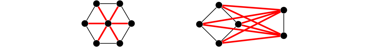
A regular graph is one in which every vertex has the same degree. The term k-regular is used to denote a graph in which every vertex has degree k. There are may types of regular graphs. Shown below are a 2-regular, a 3-regular, and a 4-regular graph.

Others

There are various other classes of graphs. A few examples are shown below. Many have fun names like caterpillars and claws. It is not necessary to learn their names at this point.

Subgraphs

A subgraph is part of a graph, where we take some of its vertices and edges. Here is the formal definition.

A graph H is a subgraph of a graph G provided the vertices of H are a subset of the vertices of G and the edges of H are a subset of the edges of G.

Shown below on the left is a graph. The two graphs to the right are subgraphs of it (with the vertices and edges that are not included in the subgraph shown in a lighter color; they are not part of the subgraph).

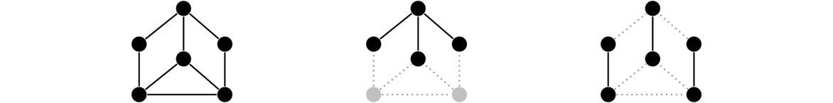
Note that if an edge is part of a subgraph, both of its endpoints must be. It doesn't make sense to have an edge without an endpoint.

Induced subgraphs

Often the subgraphs we will be interested in are induced subgraphs, where whenever two vertices are included, if there is an edge in the original graph between those two vertices, then that edge must be included in the subgraph as well.

Below on the left we have a graph followed by two subgraphs of it. The first subgraph is not induced since it includes vertices a, b, c, and d, but not all of the edges from the original graph between those vertices, such as edge bc. The second subgraph is induced.

Removing vertices

Quite often, we will want to remove vertices from a graph. Whenever we do so, we must also remove any edges incident on those vertices. Shown below is a graph and two subgraphs obtained by removing vertices.

In the middle graph we have removed the vertex a, which means we have to remove its four edges. In the right graph, we have removed vertices b and c, which has the effect of breaking the graph into two pieces.

If G is a graph and S is a subset of its vertices, we will use the notation G-S for the graph obtained by removing the vertices of S. If S consists of just a single vertex v, we will write G-v instead. And if we are removing just a single edge e from a graph, we will denote that by G-e.

Special subgraphs

Paths and cycles

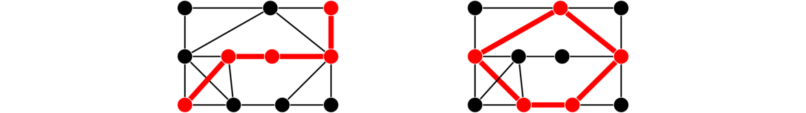
We will often be interested in paths and cycles in graphs. Any time we say a graph “contains a path” or “contains a cycle”, what we mean is that it has a subgraph that is a path or a cycle. Examples of a path and a cycle in a graph are highlighted below.

Cliques

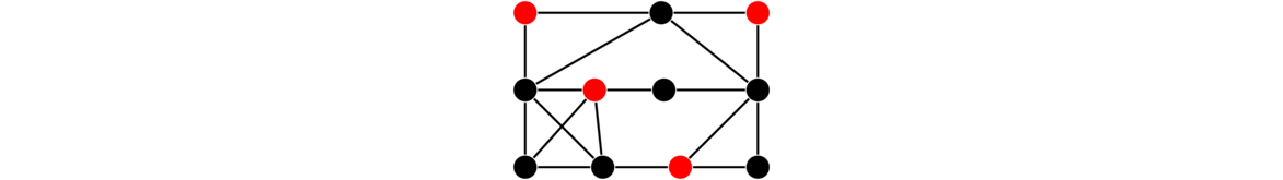
A subgraph that is a complete graph is called a clique. It is a subgraph in which every vertex in the subgraph is adjacent to every other vertex in the subgraph. For example, in the graph below we have a 4-clique in the lower left and a 3-clique (usually called a triangle) in the upper right.

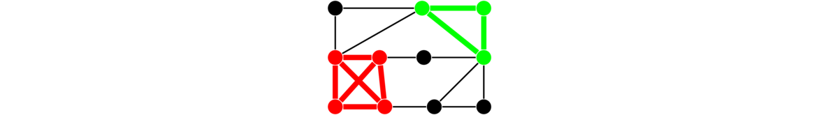
One way to think about cliques is as follows: Suppose we have a graph representing a social network. The vertices represent people, with an edge between two vertices meaning that those people know each other. A clique in this graph is a group of people that all know each other.

Independent sets

The opposite of a clique is an independent set. It is a collection of vertices in a graph in which no vertex is adjacent to any other. Keeping with the social network example, an independent set would be a collection of people that are all strangers to each other. An independent set is highlighted in the graph below.

Graph theorists are interested in the problem of finding the largest clique and largest independent set in a graph, both of which are difficult to find in large graphs.

Connectedness

Shown below on the left is a connected graph and on the right a disconnected graph.

We see intuitively that a disconnected graph is in multiple “pieces,” but how would we define this rigorously? The key feature of a connected graph is that we can get from any vertex to any other. This is how we define connectivity. Formally, we have the following:

A graph is connected provided there exists a path in the graph between any two vertices. Otherwise, the graph is disconnected.

To reiterate—the defining feature of a connected graph is that it is possible to get from any vertex to any other. Later on, when we look at proofs, if we want to prove a graph is connected, we will need to show that no matter what vertices we pick, there must be a path between them.

The pieces of a disconnected graph are called its components. For instance, in the disconnected graph above on the right, the three components are the triangle, the two vertices on the right connected by an edge, and the single vertex at the top.

Just like with connectivity, we hopefully have a clear idea of what a piece or component of a graph is, but how would we define it precisely? Before reading on, try to think about how you would define it.

One possible definition might be that a component is a connected subgraph. But that isn't quite right, as in the graph above on the right there are more than 3 connected subgraphs. For instance, the bottom part of the triangle is a connected subgraph but not a component. The trick is that a component is a connected subgraph that is as large as possible—that there is no other vertex that could be added to it and have it still remain connected.

Mathematicians use the term maximal for situations like this. A component is a maximal connected subgraph, one that cannot be made any larger and still remain connected. Here is the formal definition.

A component of a graph is a maximal connected subgraph.

Another way to think about a component is that it is a connected subgraph that is not contained in any other connected subgraph.

Note that a connected graph has one component. Also, a component that consists of a single vertex is called an isolated vertex.

Other important terminology

Cut vertices and cut edges

Here are two important types of vertices and edges.

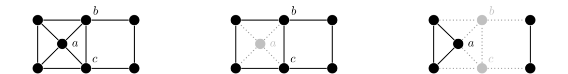
A cut vertex of a graph is a vertex which, if deleted, breaks the graph into more components than it originally had. A cut edge is defined analogously. It is an edge which, if deleted, breaks the graph into more components than it originally had.

In particular, removing a cut vertex or a cut edge from a connected graph will disconnect the graph. For example, in the graph below on the left, a, b, and c are cut vertices, as deleting any one of them would disconnect the graph. Similarly, since deleting edge bc disconnects the graph, that makes bc a cut edge. There are no other cut vertices and cut edges in the graph.

Cut vertices and cut edges act like bottlenecks when it comes to connectivity. For instance, any path in the graph above from the leftmost to the rightmost vertices must pass through a, b, c, and the edge bc.

Removing a cut vertex could break a connected graph into two components or possibly more. For instance, removing the center of a star will break it into many components. Removing a cut edge can only break a connected graph into two components.

Distance

In a graph, the distance between two vertices is a measure of how far apart they are.

The distance between two vertices, denoted d(u,v), is the length of the shortest path between u and v in the graph. It is essentially how many “steps” the vertices are away from each other.

For example, in the graph below, b, c, and d are at a distance of 1 from a. Vertex e is at distance of 2 from a, and vertex f is at a distance of 3 from a.

Notice, for instance that there are multiple paths from a to d, but the shortest path is of length 1, so that is the distance.

Graph isomorphism

The term isomorphism literally means “same shape.” It comes up in many different branches of math. In graph theory, when we say two graphs are isomorphic, we mean that they are really the same graph, just drawn or presented possibly differently. For example, the figure below shows two graphs which are isomorphic to each other.

In both graphs, each vertex is adjacent to each other vertex, so these are two isomorphic copies of K₄. For a simple example like this one, it's not too hard to picture morphing one graph into the other by sliding vertices around. But for graphs with many vertices, this approach is not feasible. It can actually be pretty tricky to show that two large graphs are isomorphic. For instance, the three graphs below are all isomorphic, and it is not at all trivial to see that.

Before we go any further, here is the formal definition:

Graphs G and H are isomorphic provided there exists a one-to-one and onto function f:V(G) → V(H) such that v is adjacent to w in G if and only if f(v) is adjacent to f(w) in H.

In other words, for two graphs to be isomorphic, we need to be able to perfectly match up the vertices of one graph with the vertices of the other, so that whenever two vertices are adjacent in the first graph, the vertices they are matched up with must also be adjacent. And if those vertices are not adjacent in the original, the vertices they are matched up with must not be adjacent either.

For example, we can use the definition to show the graphs below are isomorphic.

To do this, we match up the vertices as follows:

a ↔ v b ↔ w c ↔ x d ↔ z e ↔ y

Written in function notation, this matching is f(a) = v, f(b) = w, f(c) = x, f(d) = z, and f(e) = y. It is one-to-one and onto. We also need to check that all the edges work out. For instance, ab is an edge in the left graph. Since a and b are matched with v and w, we need vw to be an edge in the right graph, and it is. Similarly, there is no edge from a to e in the left graph. Since a and e are matched to v and y, we cannot have an edge in the right graph from v to y, and there is none. Though it's a little tedious, it's possible to check all the edges and nonedges in this way.

Showing two graphs are isomorphic can be tricky, especially if the graphs are large. If we just use the definition, there are many possible matchings we could try, and for each of those, checking that all the edges work out can take a while. There are, however, algorithms that work more quickly than this, and it is a big open question in the field of graph algorithms as to exactly how good these algorithms can be made.

On the other hand, it can often be pretty simple sometimes to show that two graphs are not isomorphic. We need to find a property that the two graphs don't share. Here is a list of a few properties one could use:

If the two graphs have a different number of vertices or edges
If the two graphs have different numbers of components
If the vertex degrees are not exactly the same in each graph
If the graphs don't contain exactly the same subgraphs

Here is an example. Both graphs below have the same number of vertices, both have the same number edges, both have one component, and both consist of two vertices of degree 1, two vertices of degree 2, and four vertices of degree 3. So the first three properties are no help. However, the right graph contains a triangle, while the left graph does not, so the fourth property comes to our rescue.

There are many other possibilities besides the four properties above. Sometimes, it takes a little creativity. For example, the graphs below are not isomorphic. Note that they do both have the same number of vertices and edges, and in fact the degrees of all the vertices are the same in both graphs. However, the right graph contains a vertex of degree 3 adjacent to two vertices of degree 1, while that is not the case in the left graph. Another way to approach this is that the left graph contains two paths of length 5 (the straight-line path along the bottom, and one starting with the top vertex and then turning left along the path), while the right graph just contains one path of length 5.

New graphs from old graphs

This section explores a few ways of using graphs to create new graphs.

Complements

The complement of a graph G is a graph G with the same vertex set as G, but whose edges are exactly the opposite of the edges in G. That is, uv is an edge of G if and only if uv is not an edge of G. Shown below are a graph and its complement.

One way to think of the complement is that the original plus the complement equals a complete graph. So we can get the complement by taking a complete graph and removing all the edges associated with the original graph.

Union

The union of two graphs is obtained by taking copies of each graph and putting them together into one graph. Formally, given graphs G and H, their union G ∪ H has vertex set V(G ∪ H) = V(G) ∪ V(H) and edge set E(G ∪ H) = E(G) ∪ E(H). The same idea works with unions of more than two graphs. For instance, shown below is C₄ ∪ K₂ ∪ K₄.

Join

The join of two graphs, G and H, is formed by taking a copy of G, a copy of H, and adding an edge from every vertex of G to every vertex of H.

For example, shown below on the left is a type of graph called a wheel, which is K₁ ∨ C₆. It consists of a 6-cycle and a single vertex, with edges from that single vertex to every vertex of the cycle. On the right we have C₄ ∨ K₂.

Formally, the join G ∨ H has vertex set V(G∨ H) = V(G) ∪ V(H) and edge set E(G∨ H) = E(G) ∪ E(H) ∪ {gh : g ∈ V(G), h ∈ V(H)}.

Line graph

The line graph, L(G), of a graph G is a graph that we create from the edges of G. Each edge of G becomes a vertex of L(G). Two vertices in L(G) are adjacent if and only if their corresponding edges in G share an endpoint. Shown below is an example of a graph and the construction of its line graph.

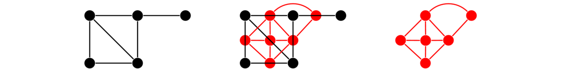
To create the line graph above, we start by making a vertex for each edge of the original graph. Then we create the edges of the line graph according to the rule above. For example, the top two edges of the original graph share an endpoint, so we will get an edge in the line graph between the vertices representing those edges. Similarly, the diagonal edge in the original shares endpoints with 4 other edges, so in the line graph it will have degree 4.

Sometimes questions about edges of G can be translated to questions about vertices of L(G).

Cartesian product

The Cartesian product graph is related to the Cartesian product of sets. The basic idea is, starting with two graphs G and H, to get the Cartesian product G □ H, we replace each vertex of G with an entire copy of H. We then add edges between two copies provided there was an edge in G between the two vertices those copies replaced. And we only add edges between the two copies between identical vertices in the copies. An example is shown below.

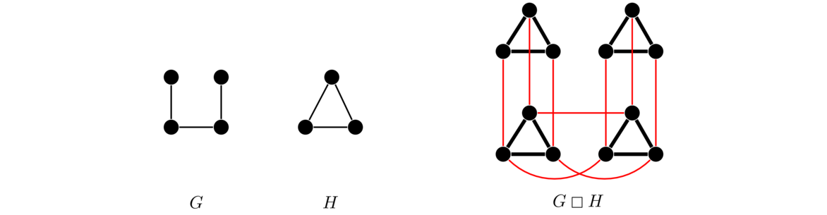
Notice how each of the four vertices of G is replaced with a copy of the triangle, H. Then wherever there is an edge in G, we connect up the triangles, and we do this by connecting up like vertices with like vertices.

Formally, the vertex set of the Cartesian product G □ H is V(G) × V(H) (that is, all pairs (v,w), with v ∈ V(G) and w ∈ V(H)). The edges of the Cartesian product are as follows: for each v ∈ V(G) there is an edge between (v,w₁) and (v,w₂) if and only if w₁w₂ ∈ E(H); and for each w ∈ V(H), there is an edge between (v₁,w) and (v₂,w) if and only if v₁v₂ ∈ E(G).

Here is another example of a Cartesian product: a grid graph. Here we have labeled the vertices with their “Cartesian coordinates.”

Hypercubes are important graphs defined by the Cartesian product. The first hypercube, Q₁ is K₂. The second hypercube, Q₂ is Q₁ □ K₂, a square. The third hypercube Q₃ is Q₂ □ K₂, which gives a graph representing an ordinary cube. In general, Q_n = Q_n-1 □ K₂ for n ≥ 2. The first four are shown below. The last one is a drawing of a 4-dimensional cube on a flat plane. It is shown with the two copies of Q₃ highlighted.

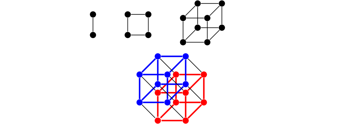
In general, each hypercube comes from two copies of the previous hypercube connected up according to the Cartesian product rules.

Note: Notice from the definition of the Cartesian product that G □ H is isomorphic to H □ G.

Proofs, Constructions, Algorithms, and Applications

Basic results and proving things about graphs

In these notes, we will cover a number of facts about graphs. It's nice to be sure that something is true and to know why it is true, and that's what a mathematical proof is for. Our proofs, like many in math, are designed to convince a mathematical reader that a result is true. To keep things succinct, we don't always include every detail, relying on the reader to fill in small gaps. The proofs themselves will often consist more of words than of symbols.

The Degree sum formula and the Handshaking lemma

Here is the first result that many people learn in graph theory.

[Degree sum formula] In any graph, the sum of the degrees of all vertices is twice the number of edges.

Every edge contributes 2 to the total degree sum, one for each of its endpoints.

Note that if we want to be a bit more formal, we can state the result above as follows:

Σ_{v ∈ V(G)} deg(v) = 2 |E(G)|.

In particular, the degree sum must be even. These leads to the following consequence, called the Handshaking lemma.

(Handshaking lemma) In every graph, there are an even number of vertices of odd degree.

If there were an odd number of vertices of odd degree, then the total degree sum would be odd, contradicting the previous theorem.

The “Handshaking lemma' comes from the following: Suppose some people at a party shake hands with others. Then there must be an even number of people who shook an odd number of hands. Here the people are vertices, with an edge between two vertices if the corresponding people shook hands.

To summarize: the sum of the degrees in any graph is twice the number of edges, and graphs with an odd number of odd-degree vertices are impossible. We will make use of these results repeatedly in these notes, so know them well.

An application of the Degree sum formula

Here is one use of the Degree sum formula.

If a graph has exactly two vertices of odd degree, then there must be a path between them.

If there were no path between the vertices, then they would lie in different components. Those components would then have exactly one vertex of odd degree each, contradicting the Handshaking lemma, as the components are themselves graphs. So there must be a path between those vertices.

The proof above, like the proof of the Handshaking lemma, is an example of a proof by contradiction. We start by assuming that the result is false, and end up contradicting something we know must be true. The conclusion then is that our result must be true. Proof by contradiction is a useful and powerful technique for proving things.

Another theorem about vertex degrees

Continuing with vertex degrees, here is another result that might be a little surprising.

In every simple graph with at least two vertices, there are at least two vertices with the same degree.

Suppose not: suppose that all n vertices have different degrees. Since the graph is simple, the largest possible degree of a vertex is n-1. Since all the degrees are different, those degrees must be 0, 1, 2, …, n-1, with exactly one vertex of each degree. A vertex with degree 0 is adjacent to nothing, and a vertex with degree n-1 is adjacent to every vertex except itself. But these statements are incompatible with each other. A graph can't contain both a vertex adjacent to every other vertex and a vertex adjacent to nothing. So we have a contradiction, meaning that some vertices must share the same degree.

Sometimes, with proofs like these, it helps to look at a specific example. Suppose we have n = 5 vertices. Then if the degrees are all different, the degrees must be 0, 1, 2, 3, and 4. That degree 4 vertex is adjacent to all of the others, including the degree 0 vertex, which isn't possible. So the degrees must be five integers in the range from 0 to 3 or five integers in the range from 1 to 4, meaning there will be a repeated degree.

Notice where in the proof the fact that the graph is simple is used—namely, in guaranteeing that we have to have a vertex adjacent to all others along with a vertex of degree 0. If we remove the requirement that the graph be simple and allow loops and multiple edges, then the result turns out to be false. It's a nice exercise to try to find counterexamples in that case.

Notice also that we use a proof by contradiction here again. Some mathematicians (but not this author) feel that proofs by contradiction are poor mathematical style and that direct proofs should be preferred. The proof above could be reworked into a direct proof using the pigeonhole principle. It's another nice exercise to try to do that.

A proof about connectedness

To get some more practice with proofs, here is another result, this one about connectedness.

If a graph is disconnected, then its complement is connected.

Call the graph G. Since it is disconnected, it has to have at least two vertices. Pick any two vertices u and v. We need to show that there is a path between them in G. First, if u and v are different components of G, then uv∉ E(G), which means uv ∈ E(G) and hence we have a path from u to v in G. On the other hand, if u and v are in the same component of G, then pick some other vertex w in a different component. Then uw and wv are not in E(G), meaning they are in E(G). Thus we have a path in G between u and v that goes through w.

The proof is only a couple of lines, but a fair amount of thinking and work goes into producing those lines. To start, we go straight to the definition of connectedness. Specifically, to show G is connected, we have to show there is a path between any two vertices. Let's call them u and v, as we did in the proof. Next, it helps to draw a picture. We know that G is disconnected, so we might try a picture like the one below.

The picture shows two components, though there might be more. We know that when we take the complement, any two components of the original will be joined together by all possible edges between vertices. So if u and v started out in different components, they would be adjacent in the complement. So that's one case taken care of. But now what if u and v are in the same component? We can't forget about that case.

If u and v are in the same component, then there is a path between them in G, but maybe they end up separated when we take the complement. This turns out not to be a problem. Recall that we have all possible edges between any two components, so we can create a two-step path from u to v by jumping from u to some vertex w in a different component and then back to v.

To summarize: We are trying to find a path between any two vertices u and v in G. We have broken things into two cases: one where u and v are in different components, and one where u and v are in the same component. When doing proofs, it is often useful to break things into cases like this. And it is important to make sure that every possible case is covered.

The theorem above says that the complement of a disconnected graph is connected. What if we try changing it around to ask if the complement of a connected graph is disconnected? It turns out not to be true in general. To show this we need a single counterexample, like the one below, showing C₅ and its complement, both of which are connected.

In general, to prove something requires a logical argument, while to disprove something requires just a single counterexample.

An if-and-only-if proof

Here is another statement, this one a biconditional (if-and-only-if statement).

An edge in a graph is a cut edge if and only if it is part of no cycle.

It is essentially two statements in one, meaning there are two things to prove, namely:

If e is a cut edge, then it is part of no cycle.
If e is part of no cycle, then it is a cut edge.

It basically says that being a cut edge is equivalent to not being a part of a cycle. Those two concepts can be used interchangeably. Here is the proof of the theorem:

Call the graph G, call the cut edge e, and let its endpoints be called u and v.

First, assume e is a cut edge. Then deleting it breaks the graph into more than one component, with u in one component and v in another. Suppose e were part of a cycle. Then going the other way along the cycle from u to v, avoiding edge e, would provide a path from u to v, meaning those vertices are in the same component, a contradiction. Thus e cannot be part of a cycle.

Next, assume e is part of no cycle. Then there cannot be any path between u and v other than along edge e, as otherwise we could combine that path along with e to create a cycle. Thus, if we delete e, there is no path from u to v, meaning u and v are in different components of G-e. So e is a cut edge.

Often when trying to understand a proof like this, or in trying to come up with it yourself, it helps to draw a picture. Here is a picture to help with visualizing what happens in the proof.

Mathematical induction

Consider the following problem: Alice and her husband Bob are at a party with 3 other couples. At the party some people shake hands with some others. No one shakes their own hand or the hand of their partner. Alice asks everyone else how many hands they each shook, and everyone gives a different answer. How many different hands did Bob shake?

This seems like a bizarre question, like it shouldn't be answerable. Nevertheless, let's start by modeling it with a graph. The people become vertices and edges indicate handshakes. The degree of a vertex is how many hands that vertex's corresponding person shook. See below on the left for what our graph initially looks like.

There are 4 couples and 8 people total. Alice asks the other 7 people and gets 7 different answers. That means the answers must be the integers from 0 to 6. Let p₀, p₁, …, p₆ be the names of the people that shook 0, 1, …, 6 hands, respectively.

Person p₆ must have shaken hands with everyone at the party except p₆ and the partner of p₆. That means that the partner of p₆ must be p₀, since everyone else must have shaken at least one hand (namely the hand of p₆).

It's important to note that p₆ can't be Bob. Why? Since p₆ shakes hands with everyone except themselves and their partner, that means there can't be any other vertex with degree 0 in the graph besides the partner of p₆. If Bob were p₆, then both p₀ and Alice (who is not one of the p_i) would have to shake 0 hands.

Now consider p₅. That person shook hands with everyone except p₅, the partner of p₅ and p₀. This means that p₁ must be the partner of p₅, since everyone else must have shaken at least two hands (namely the hands of p₅ and p₆. And by the same argument as above, p₁ and p₅ are not Alice and Bob.

A similar argument to the ones we have just looked at show that p₄ and p₂ are partners and they are not Alice and Bob. This means that Bob must be p₃, having shaken 3 hands. The graph of this ends up looking like the one above on the right.

The general case

Suppose we generalize this to a party of n couples. How many hands must Bob have shaken in that case? The answer is n-1. We can show this by generalizing and formalizing the argument above using mathematical induction. As above, we model the party by a graph where the people are vertices and edges indicate handshakes.

The base case is a party with n = 1 couple, just Alice and Bob. Since they are partners, they don't shake each other's hands. So Bob shakes no hands, which is the same as n-1 with n = 1.

Now assume that at any party of n couples satisfying the setup of the problem, Bob shakes n-1 hands. Consider then a party of n+1 couples. We need to show that Bob shakes exactly n hands in this party.

Since the answers that Alice gets are all different, they must be the integers from 0 through 2n. Let p₀, p₁, …, p_2n be the names of the people that shook 0, 1, …, 2n hands, respectively. Then p_2n must have shaken hands with everyone else at the party except p_2n and the partner of p_2n. That is, vertex p_2n is adjacent to all vertices of the graph except itself and one other vertex. That other person/vertex, must be p₀. So p_2n and p₀ are partners. As before, p₀ and p_2n cannot be Alice and Bob (or Bob and Alice).

Now remove p₀ and p_2n from the party/graph. Doing so leaves a graph corresponding to n couples, where the degree of each vertex has been reduced by exactly 1. This party/graph satisfies the induction hypothesis—namely, it is a party of n couples and everyone that Alice asks has a different degree because their degrees were all different in the original and we have subtracted precisely 1 from all of those degrees.

By the induction hypothesis, Bob must have shaken n-1 hands among this party. Therefore in the original party, Bob shook n hands, those being the n-1 in the smaller party along with the hand of p_2n.

A little about induction

If you have never seen induction, then the preceding may likely make no sense to you. Consider picking up a book on Discrete Math to learn some induction. But even if you have seen induction before, the preceding may seem odd. It almost seems like cheating, like we didn't really prove anything. The key here is the work that goes into setting the proof up. In particular, when we remove a couple from the graph to get to the smaller case, we can't remove just any couple. We need to remove a couple that preserves the parameters of the problem, especially the part about Alice getting all different answers. The hard work comes in planning things out. The finished product, the proof, ends up relatively short.

Constructions

Often we will want to build a graph that has certain properties. This section contains a few examples.

Constructing a multigraph with given degrees

The first question we will answer is this: given a sequence of integers, is there a multigraph for which those integers are the degrees of its vertices? The answer is yes, provided the sequence satisfies the Handshaking lemma, namely that there must be an even amount of odd integers in the sequence. We can show this by constructing the graph.

To see how it works, it helps to use an example. Let's take the sequence 0, 2, 3, 3, 5, 7, 8. Start by creating one vertex for each integer in the sequence. Then pair off the first two odd integers, 3 and 3, and add an edge between their corresponding vertices. Then do the same for the other two odd integers, 5 and 7. Adding the edges between pairs of odd degree vertices essentially takes care of the “odd part” of their degrees, leaving only an even number to worry about. We can use loops to take care of those even numbers since each loop adds 2 to a vertex's degree. See the figure below for the process.

This technique works in general. We start by pairing off the first two odd integers and adding an edge between their vertices, then pairing off the next two odd integers, etc. until we have worked through all the odd integers. It's possible to pair off all the odds since we know there must be an even number of them by the Handshaking lemma. After doing this, add loops to each vertex until its degree matches it sequence value.

Constructing regular graphs

Our second example is to answer the following question: given integers r and n, is it possible to construct an r-regular simple graph with n vertices? The answer is yes provided r ≤ n-1 and at least one of r and n is even. We need r ≤ n-1 since n-1 is the largest degree a vertex can have in a simple graph, and we need at least one of r and n to be even by the Handshaking lemma.

The construction is different depending on if r is even or odd. We'll do the even case first. Start by placing n vertices around a circle. This is a 0-regular graph on n vertices. To create a 2-regular graph from it, join each vertex to its two neighbors. The graph created this way is the cycle C_n. To create a 4-regular graph, join each vertex additionally to both vertices that are at a distance of 2 from it along the circle. To create a 6-regular graph, join each vertex to both vertices that are at a distance of 3 from it along the circle. This same idea can be extended to create larger regular graphs of even degree. The graph below on the left is an example of the 4-regular graph on 12 vertices created by this process.

To create a regular graph of odd degree, use the exact same process, but additionally connect each vertex to the vertex on the circle diametrically opposite to it. Shown above on the right is a 5-regular graph on 12 vertices. Note that in the figure, the lines all cross at the center, giving the illusion of a vertex there, but there is not one.

It is worth describing this construction formally. Here is one way to do it: Call the vertices v₀, v₁, …, v_n-1. For an r-regular graph, where r is even, for each vertex v_i, add edges from v_i to v_{(i± k) mod n}, for k = 1, 2, … r/2. If r is odd, add all of those edges along with an edge from v_i to v_{(i+n/2) mod n}.

These graphs are called Harary graphs, after the graph theorist Frank Harary.

Graph Representations

Graph theory has a lot of applications to real problems. Those problems often are described by graphs with hundreds, thousands, or even millions of vertices. For graphs of that size, we need a way of representing them on a computer. There a two ways this is usually done: adjacency matrices and adjacency lists.

Adjacency matrix

The idea is that we use a matrix to keep track of which vertices are adjacent to which other vertices. An entry of 1 in the matrix indicates two vertices are adjacent and a 0 indicates they aren't adjacent. For instance, here is a graph and its adjacency matrix:

Adjacency lists

The second approach to implementing a graph is to use adjacency lists. For each vertex of the graph we keep a list of the vertices it is adjacent to. Here is a graph and its adjacency lists:

Adjacency matrices vs. adjacency lists

Adjacency matrices make it very quick to check if two vertices are adjacent. However, if the graph is very large, adjacency matrices can use a lot of space. For instance, a 1,000,000 vertex graph would require 1,000,000 × 1,000,000 entries, having a trillion total entries. This would require an unacceptably large amount of space.

Adjacency lists use a lot less space than adjacency matrices if vertex degrees are relatively small, which is the case for many graphs that arise in practice. For this reason (and others) adjacency lists are used more often than adjacency matrices when representing a graph on a computer.

Coding a graph class

Here is a quick way to create a graph class in Python using adjacency lists:

class Graph(dict):
    def add(self, v):
        self[v] = set()

    def add_edge(self, u, v):
        self[u].add(v)
        self[v].add(u)

One thing worth noting is that we are actually using adjacency sets instead of lists. It's not strictly necessary, but it does make a few things easier later on. The class inherits from the Python dictionary class, which gives us a number of useful things for free. For instance, if our graph is called G with a vertex 'a', then G['a'] will give us the neighbors of that vertex. We have created two methods for the class. The first one adds a vertex. To do so, it creates an entry in the dictionary with an empty adjacency list (set). The other method is for adding an edge. We do that by adding each endpoint to the other endpoint's adjacency list.

Below is an example showing how to create a graph and add some vertices and edges:

G = Graph()
G.add('a')
G.add('b')
G.add('c')
G.add_edge('a', 'b')
G.add_edge('a', 'c')

Here is a quicker way to add a bunch of vertices and edges:

G = Graph()
for v in 'abcde':
    G.add(v)
for e in 'ab ac bc ad de'.split():
    G.add_edge(e[0], e[1])

Below we show how to print a few facts about the graph:

print(G)
print('Neighbors of a: ', G['a'])
print('Degree of a:', len(G['a']))
print('Is there a vertex z?', 'z' in G)
print('Is there an edge from a to b?', 'b' in G['a'])
print('Number of vertices:', len(G))
for v in G:    # loop over and print all the vertices
    print(v)

Algorithms

One of the most important parts of graph theory is the study of graph algorithms. An algorithm is, roughly speaking, a step-by-step process for accomplishing something. For instance, the processes students learn in grade school for adding and multiplying numbers by hand are examples of algorithms. In graph theory, there are algorithms to find various important things about a graph, like finding all the cut edges or finding the shortest path between two vertices.

One of the most fundamental tasks on a graph is to visit the vertices in a systematic way. We will look at two related algorithms for this: breadth-first search (BFS) and depth-first search (DFS). The basic idea of each of these is we start somewhere in the graph, then visit that vertex's neighbors, then their neighbors, etc., all the while keeping track of vertices we've already visited to avoid getting stuck in an infinite loop.

The figure below shows the order in which BFS and DFS visit the vertices of a graph, starting at vertex a. Assume that when choosing between neighbors, it goes with the one that is alphabetically first.

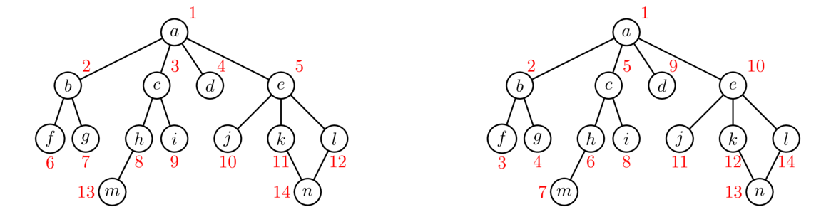
Notice how BFS fans out from vertex a. Every vertex at distance 1 from a is visited before any vertex at distance 2. Then every vertex at distance 2 is visited before any vertex at distance 3. DFS, on the other hand, follows a path down into the graph as far as it can go until it gets stuck. Then it backtracks to its previous location and tries searching from there some more. It continues this strategy of following paths and backtracking.

These are the two key ideas: BFS fans out from the starting vertex, doing a systematic sweep. DFS just goes down into the graph until it gets stuck, and then backtracks. If we are just trying to find all the vertices in a graph, then both BFS and DFS will work equally well. However, if we are searching for vertices with a particular property, then depending on where those vertices are located in relation to the start vertex, BFS and DFS will behave differently. BFS, with its systematic search, will always find the closest vertex to the starting vertex. However, because of its systematic sweep, it might take BFS a while before it gets to vertices far from the starting vertex. DFS, on the other hand, can very quickly get far from the start, but will often not find the closest vertex first.

Code for BFS

In both BFS and DFS, we start at a given vertex and see what we can find from there. The searching process consists of visiting a vertex, looking at its neighbors, and adding any new neighbors to two separate lists. One list (actually a set) is for keeping track of what vertices we have already found. The other list keeps track of the order we will visit vertices to see what their neighbors are. Here is some code implementing BFS:

def bfs(G, start):
    found = {start}
    waiting = [start]

    while waiting:
        w = waiting.pop(0)
        for n in G[w]:
            if n not in found:
                found.add(n)
                waiting.append(n)
    return found

The function takes two parameters: a graph G and a vertex start, which is the vertex we start the search at. We maintain a set called found that remembers all the vertices we have found, and we maintain a list called waiting that keeps of the vertices we will be visiting. It acts like a queue. Initially, both start out with only start in them. We then continually do the following: pop off a vertex from the waiting list and loop through its neighbors, adding any neighbor we haven't already found into both the found set and waiting list.

The while loop keeps running as long as the waiting list is not empty, i.e. as long as there are still vertices we haven't explored. At the end, we return all the vertices that were discovered by the search.

Let's run BFS on the graph below, starting at vertex a. The first thing the algorithm does is add each of the neighbors of a to the waiting list and found set. So at this point, the waiting list is [b,c,d,e]. BFS always visits the first vertex in the waiting list, so it visits b next and adds its neighbors to the list and set. So now the waiting list is [c,d,e,f,g]. For the next step, we take the first thing off the waiting list, which is c and visit it. We add its neighbors h and i to the list and set. This gives us a waiting list of [d,e,f,g,h,i]. As the process continues, the waiting list will start shrinking and the found set will eventually include all the vertices.

Note that the code has been deliberately kept small. It has the effect of finding all the vertices that can be reached from the starting vertex. We will soon see how to modify this code to do more interesting things.

Also note that We could use a list for found instead of a set, but the result would be substantially slower for large graphs. The part where we check to see if a vertex is already in the found set is the key. The algorithm Python uses to check if something is in a set is much faster than the corresponding list-checking algorithm.

Code for DFS

One way to implement DFS is to use the exact same code as BFS except for one extremely small change: Use waiting.pop() instead of waiting.pop(0). Everything else stays the same. Using waiting.pop() changes the order in how we choose which vertex to visit next. DFS visits the most recently added vertex, while BFS visits the earliest added vertex. BFS treats the list of vertices to visit as a queue, while DFS treats the list as a stack. Here is the code:

def dfs(G, start):
    found = {start}
    waiting = [start]

    while waiting:
        w = waiting.pop()
        for n in G[w]:
            if n not in found:
                found.add(n)
                waiting.append(n)
    return found

Though it works, it's probably not the best way to implement DFS. Recall that DFS works by going as down in the tree until it gets stuck, then backs up one step, tries going further along a different path until it gets stuck, backs up again, etc. One benefit of this approach is that it doesn't require too much memory. The search just needs to remember info about the path it is currently on. The code above, on the other hand, adds all the neighbors of a vertex into the waiting list as soon as it finds them. This means the waiting list can grow fairly large, like in BFS. Below is a different approach that avoids this problem.

def dfs(G, start):
    waiting = [start]
    found = {start}

    while waiting:
        w = waiting[-1]
        N = [n for n in G[w] if n not in found]
        if len(N) == 0:
            waiting.pop()
        else:
            n = N[0]
            found.add(n)
            waiting.append(n)
    return found

You'll often see DFS implemented recursively. It's probably more natural to implement it that way. Here is a short function to do just that:

def dfs(G, w, found):
    found.add(w)
    for x in G[w]:
        if x not in found:
            dfs(G, x, found)

We have to pass it a set to hold all the vertices it finds. For instance, if we're starting a search at a vertex labeled 'a', we could create the set as S = {'a'} and then call dfs(G, 'a', S).

Applications of BFS and DFS

The algorithms as presented above act as something we can build on for more complex applications. Small modifications to them will allow us to find a number of things about a graph, such as a shortest path between two vertices, the graph's components, its cut edges, and whether the graph contains any cycles.

As an example, here is a modification of BFS to determine if there is a path between two vertices in a graph:

def is_connected_to(G, u, v):
    found = [u]
    waiting = [u]

    while waiting:
        w = waiting.pop(0)
        for x in G[w]:
            if x == v:
                return True
            elif x not in found:
                found.append(x)
                waiting.append(x)
    return False

The main change is when we look at neighbors, if the vertex we are looking for shows up, then we stop immediately and return True. If we get all the way through the search and haven't found the vertex, we return False.

Shortest path

Here is another example, this one a modification to BFS to return the shortest path between two vertices in a graph. The key difference between this code and the BFS code is that we replace the found set with a Python dictionary that keeps track of each vertex's parent. That is, instead of keeping track only of the vertices that we have found, we also keep track of what vertex we were searching from at the time. This allows us, once we find the vertex we are looking for, to backtrack from vertex to vertex to give the exact path.

def shortest_path(G, u, v):
    waiting = [u]
    found = {u : None}  # A dictionary instead of a set

    while waiting:
        w = waiting.pop(0)
        for x in G[w]:
            if x == v: # If we've found our target, then backtrack to get path
                Path = [x]
                x = w
                while x != None:
                    Path.append(x)
                    x = found[x]
                Path.reverse()
                return Path

            if x not in found:
                found[x] = w
                waiting.append(x)

    return [] # return an empty list if there is no path between the vertices

Note also that we use BFS here and not DFS. Remember that BFS always searches all the vertices at distance 1, followed by all the vertices at distance 2, etc. So whatever path it finds is guaranteed to be the shortest. Replacing BFS with DFS here would give still us a path between the vertices, but it could be long and meandering.

Components

The basic versions of BFS and DFS that we presented return all the vertices in the same component as the starting vertex. With a little work, we can modify this to return a list of all the components in the graph. We do this by looping over all the vertices in the graph and running a BFS or DFS using each vertex as a starting vertex. Of course, once we know what component a vertex belongs to, there is no sense in running a search from it, so in our code we'll skip vertices that we have already found. Here is the code:

def components(G):
    component_list = []
    found = set()
    for w in G:
        if w in found:  # skip vertices whose components we already know
            continue

        # now run a BFS starting from vertex w
        found.add(w)
        component = [w]
        waiting = [w]

        while waiting:
            v = waiting.pop(0)
            for u in G[v]:
                if u not in found:
                    waiting.append(u)
                    component.append(u)
                    found.add(u)
        component_list.append(component)
    return component_list

Applications of graphs

Graphs lend themselves to solving a wide variety of problems. We will see a number of applications in later chapters. In this section we introduce a few applications of material we have already covered.

Graph theory for solving an old puzzle

This first application doesn't really apply to the real world, but it does demonstrate how we can model something with a graph. It is about the following puzzle that is over 1000 years old:

A traveler has to get a wolf, a goat, and a cabbage across a river. The problem is that the wolf can't be left alone with the goat, the goat can't be left alone with the cabbage, and the boat can only hold the traveler and a single animal/vegetable at once. How can the traveler get all three items safely across the river?

To model this problem with a graph, it helps to think of the possible “states” of the puzzle. For example, the starting state consists of the traveler, wolf, goat, and cabbage all on one side of the river with the other side empty. We can represent this state by the string “Twgc|”, where T, w, g, and c stand for the traveller, wolf, goat, and cabbage. The vertical line represents the river. The state where the wolf and cabbage are on the left side of the river and the traveller and goat are on the right side would be represented by the string “wc|Tg”.

To model this as a graph, each state/string becomes a vertex, and we have an edge between two vertices provided it is possible, following the rules of the puzzle, to move from the state represented by the one vertex to the state represented by the other in one crossing. For instance, we would have an edge between Twgc| and wc|Tg, because in we can get from one to the other in one crossing by sending the traveler and the goat across the river. Shown below is the graph we obtain.

We have omitted impossible states, like wg|Tc, from the graph above. Once we have a graph representation, we could use an algorithm like DFS or BFS to search for a path from the starting state, Twgc|, to the ending state, |Twgc. Now obviously that would be overkill for this problem, but it could be used for a more complex puzzle.

For example, you may have seen the following water jug problem: You have two jugs of certain sizes, maybe a 7-gallon and an 11-gallon jug, and you want to use them to get exactly 6 gallons of water. You are only allowed to (1) fill up a pail to the top, (2) dump a pail completely out, or (3) dump the contents of one pail into another until the pail is empty or the other is full. There is no estimating allowed.

To model this as a graph, the vertices are states which can be represented as pairs (x,y) indicating the amount of water currently in the two jugs. Edges represent valid moves. For instance, from the state (5,3), one could go to (0,3) or (5,0) by dumping out a pail, one could go to (7,3) or (5,11) by filling a pail up, or one could go to (0,8) by dumping the first into the second. One note is that these edges are one-way edges. We will cover those later when we talk about digraphs. But the main point is that with a little work, we can program in all the states and the rules for filling and emptying pails, and then run one of the searching algorithms to find a solution.

This technique is useful a number of other contexts. For instance, many computer chess-playing programs create a graph representing a game, where the states represent where all the pieces are on the board, and edges represent moves from one state to another. The program then searches as far out in the graph as it can go (it's a big graph), ranking each state according to some criteria, and then choosing its favorite state to move to.

Graphs and movies

From the International Movie Database (IMDB), it is possible to get a file that contains a rather large number of movies along with the people that have acted in each movie. A fun question to ask is to find a path from one actor X to another Y, along the lines of X acted in a movie with A who acted in a movie with B who acted in a movie with Y. There are all sorts of things we could study about this, such as whether it is always possible to find such a path or what the length of the shortest path is.

We can model this as a graph where each actor gets a vertex and each movie also gets a vertex. We then add edges between actors and the movies they acted in. The file is structured so that on each line there is a movie name followed by all the actors in that movie. The entries on each line are separated by slashes, like below:

     Princess Bride, The (1987)/Guest, Christopher (I)/Gray, Willoughby/Cook, ...

Here is some code that parses through the file and fills up the graph:

G = Graph()
for line in open('movies.txt'):
    line = line.strip()
    L = line.split('/')
    G.add(L[0])
    for x in L[1:]:
        if x not in G:
            G.add(x)
        G.add_edge(L[0], x)

We can then use a modified BFS to find the shortest path between one actor and another. Asking whether it is always possible to find a path is the same as asking whether the graph is connected. It turns out not to be, but it is “mostly” connected. That is, we can run a variation of BFS or DFS to find the components of the graph, and it turns out that the graph has one very large component, containing almost all of the actors and movies you have ever heard over. The graph contains a few dozen other small components, corresponding to isolated movies all of whose actors appeared only in that movie and nowhere else.

Word ladders

A word ladder is a path from one word to another by changing one letter at a time, with each intermediate step being a real word. For instance, one word ladder from this to that is this → thin → than → that.

We can model this as a graph whose vertices are words, with edges whenever two words differ by a single letter. Here is the code to build up a graph of four-letter words. For it, you'll need to find a list of words with one word per line. There are many such lists online.

words = [line.strip() for line in open('wordlist.txt')]
words = set(w for w in words if len(w)==4)
alpha = 'abcdefghijklmnopqrstuvwxyz'

G = Graph()
for w in words:
    G.add(w)

for w in words:
    for i in range(len(w)):
        for a in alpha:
            n = w[:i] + a + w[i+1:]
            if n in words and n != w:
                G.add_edge(w, n)

The trickiest part of the code is the part that adds the edges. To do that, for each word in the list, we try changing each letter of the word to all possible other letters, and add an edge whenever the result is a real word. Once the graph is built, we can call one of the searches to find word ladders, like below:

print(shortest_path(G, 'wait', 'lift'))

It is also interesting to look at the components of this graph. The list of words I used had 2628 four-letter words. The graph has 103 components. One of those components is 2485 words long, indicating that there is a word ladder possible between most four-letter words. Of the other components, 82 of them had just one word. Words in these components include void, hymn, ends, and onyx. The remaining components contain between 2 and 6 words, the largest of which contains the words achy, ache, ashy, acme, acne, and acre.

Real applications

The applications presented here are of more of a fun than a practical nature, but don't let that fool you. Graph theory is applied to real problems in many fields. Here is a very small sample: isomer problems in chemistry, DNA sequencing problems, flood fill in computer graphics, and matching organ donors to recipients. There are also many networking examples such as real and simulated neural networks, social networks, packet routing on the internet, where to locate web servers on a CDN, spread of disease, and network models of viral marketing.

Bipartite Graphs and Trees

Bipartite graphs

Shown below are a few bipartite graphs.

Notice that the vertices are broken into two parts: a top part and a bottom part. Edges are only possible between the two parts, not within a part, with the top and bottom parts both being independent sets. Here is the formal definition of a bipartite graph:

A bipartite graph is a graph whose vertex set can be written as the union of two disjoint sets X and Y, called partite sets, such that every edge of the graph has one endpoint in X and the other in Y.

In short, in a bipartite graph, it is possible to break the vertices into two parts, with edges only going between the parts, never inside of one. We typically draw bipartite graphs with the X partite set on top and the Y partite set on the bottom, like in the examples above. However, many graphs that are not typically drawn this way are bipartite. For example, grids are bipartite, as can be seen in the example below.

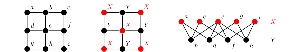
How to tell if a graph is bipartite

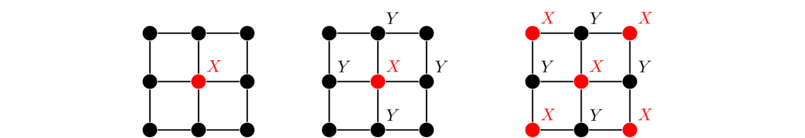
The approach to telling if a graph is bipartite is this: Start at any vertex and label it with an X. Label each of its neighbors with a Y. Label each of their neighbors with an X. Keep doing this, visiting each vertex in the graph, labeling its neighbors with the opposite of its own label. If it ever happens that two adjacent vertices get the same label or that some vertex ends up labeled with both an X and a Y, then the graph is not bipartite. If we get through every vertex without this happening, then the graph is bipartite, with the vertices labeled X and the vertices labeled Y forming the two parts of the bipartition. An example is shown below, starting at the middle vertex.

This can be coded using the BFS/DFS code from the last chapter to visit the vertices.

Suppose we try the algorithm on the triangle C₃. We start by labeling the top vertex with an X. Then its two neighbors get labeled with Y, and we have a problem because they are adjacent. A similar problem happens with C₅. See below.

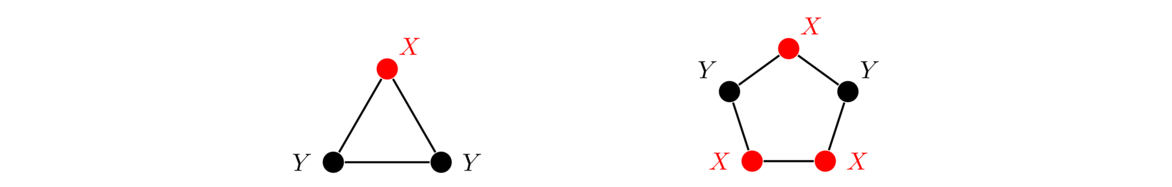
In fact, any odd cycle suffers from this problem, meaning that no odd cycle can be bipartite.

So bipartite graphs can't have odd cycles. What is remarkable is that odd cycles are the only thing bipartite graphs can't have. Namely, any graph without any odd cycles must be bipartite.

A graph is bipartite if and only if it has no odd cycles.

First, if a graph is bipartite, any cycle must have an even length. To see this, start by assuming the two partite sets are named X and Y. Pick any cycle in the graph. As we trace from vertex to vertex along that cycle, we alternate between vertices of X and vertices of Y. Suppose we start tracing at a vertex of X. Then the second, fourth, sixth, etc. vertices we meet are in X and the others are in Y. Thus when we return to our starting vertex, we have gone an even number of steps, meaning the cycle has an even length. See the figure below for an example. The labels indicate the order in which we trace around the cycle.

Now suppose we have a graph with no odd cycles. Pick any component of the graph and pick any vertex a in that component. Let X be all the vertices in the component at an even distance from a and let Y be all the vertices in the component at an odd distance from a. We claim this forms a bipartition of the component. To show this, it suffices to show there are no edges within X or within Y.

Suppose there were such an edge between vertices u and v, with both in X or both in Y. So u and v are both either at an even distance from a or both at an odd distance from a. Recall that the distance between vertices is the length of the shortest path between them. Consider the shortest paths from a to u and from a to v. These paths might share some vertices. Let b be the last vertex those paths have in common (which might possibly just be a itself). The parts of the two paths that go from a to b must have the same length or else we could use the shorter one to shorten the other's path from a to either u or v, contradicting that it's already the shortest.

The path from b to u followed by edge uv, followed by the path from v to b forms a cycle. Its length is 1 plus the distance from b to u plus the distance from b to v, and this must be odd since the distances from b to u and from b to v must both be odd or both be even, meaning their sum is even. This is a contradiction, so there cannot be any edge within X or within Y. Thus X and Y form a bipartition of the component. We can do this same process for every component to get a bipartition of the entire graph.

The picture below shows an example of the odd cycle created in the second part of the proof.

The second part of the proof relies on a clever idea, that of picking a vertex and breaking the graph into two groups: vertices that are an even distance from it and vertices that are an odd distance from it. If you want to remember how the proof goes, just remember that key idea, and the rest consists of a little work to make sure that the idea works. Many theorems in graph theory (and math in general) are like this, where there is one big idea that the proof revolves around. Learn that idea and you can often work out the other small details to complete the proof.

Relationship between the algorithm and the theorem

Usually when there is a nice characterization of something in graph theory like this, there is a simple algorithm that goes along with it. That is the case here. Though we won't do it here, it's not too hard to adapt the proof above to show that the algorithm of the previous section correctly tells if a graph is bipartite.

More on bipartite graphs

Bipartite graphs have a number of applications, some of which we will see later.

A particularly important class of bipartite graphs are complete bipartite graphs. These are bipartite graphs with all possible edges between the two parts. The notation K_m,n denotes a complete bipartite graph with one part of m vertices and the other of n vertices. Shown below are K_3,4, K_2,5, and K_3,3.

Bipartite graphs are a special case of multipartite graphs, where instead of two partite sets there can be several. For instance, shown below is a complete multipartite graph with four parts.

Trees

Trees are graphs that have a variety of important applications in math and especially computer science. Shown below are a few trees.

Trees have a certain tree-like branching to them, which is where they get their name. It is a little tricky to define a tree in terms of this branching idea. A simpler definition is the following:

A tree is a connected graph with no cycles.

From this definition, the following properties follow:

In any tree, there is exactly one path from every vertex to every other vertex.
Trees have the least number of edges a graph can have and still be connected. In particular, every edge of a tree is a cut edge.
Trees have the most number of edges a graph can have without having a cycle. In particular, adding any edge to a tree creates exactly one cycle.
Every tree with n vertices has exactly n-1 edges.

We won't formally prove the first three, but here are a few reasons why they are true:

Regarding the first property, if there were two paths to a vertex, then we could combine them to get a cycle. Regarding the second property, recall that Theorem 6 says cut edges are precisely those edges that don't lie on a cycle. For the third property, if you add an edge between vertices u and v, that would create a cycle involving edge uv and the path that is guaranteed to exist between u and v.

Leaves and induction

The last property of the previous section provides a nice opportunity to use induction. But first, we need the following definition and theorem.

A leaf in a tree is a vertex of degree 1.

That is, leaves are the vertices that are at the ends of a tree. A leaf has only one neighbor. And every nontrivial tree has a leaf, as stated below.

Every tree with at least two vertices has at least two leaves.

Consider any path of maximum length in the tree. Because the tree has at least two vertices and is connected, this path must exist. Both of the endpoints of that path are of degree 1 in the tree, with their only neighbors being the vertices immediately next to them on the path. They can have no other neighbors on the path since that would create a cycle, which is impossible in a tree. And they can have no other neighbor outside of the path since then we could have used such a neighbor to extend the path, which is impossible as the path is already maximum length.

We will use this fact and induction now to prove that every tree with n vertices has exactly n-1 edges.

The base case of a tree on one vertex with no edges fits the property. Now assume that all trees on n vertices contain n-1 edges. Let T be a tree on n+1 vertices. By Theorem 8, T has a leaf v. The graph T-v has n vertices and is a tree since removing a vertex cannot create a cycle, and removing a leaf cannot disconnect the graph. So by the induction hypothesis, T-v has n-1 edges. Since one edge was removed from T to get T-v, T must have n edges. Thus the result is true by induction.

This technique of pulling off a leaf in an induction proof is useful in proofs involving trees.

Alternate definitions of trees

Any of the tree properties mentioned earlier can themselves be used to reformulate the definition of a tree.

The following are equivalent for a graph T:

T is a tree.
Every pair of vertices of T is connected by exactly one path.
T is connected and removing any edge disconnects it.
T has no cycles and adding any edge creates a cycle.
T is connected graph with n vertices and n-1 edges.
T is an acyclic graph with n vertices and n-1 edges.

The proof of any part of this is not difficult and involves arguments similar to those we gave earlier. In addition to these, there are other ways to combine tree properties to get alternate characterizations of trees.

Forests

If we remove connectedness from the definition of a tree, then we have what is called a forest.

A forest is a graph with no cycles.

So, technically, a tree is also a forest, but most of the time, we think of a forest as a graph consisting of several components, all of which are trees (as you might expect from the name forest). A forest is shown below.

More about trees

Trees and forests are bipartite. By definition, they have no cycles, so they have no odd cycles, making them bipartite by Theorem 7.

Trees have innumerable applications, especially in computer science. There, rooted trees are the focus. These are trees where one vertex is designated as the root and the tree grows outward from there. With a root it makes sense to think of vertices as being parents of other vertices, sort of like in a family tree. Of particular interest are binary trees, where each vertex has at most two children. Binary trees are important in many algorithms of computer science, such as searching, sorting, and expression parsing.

Spanning trees

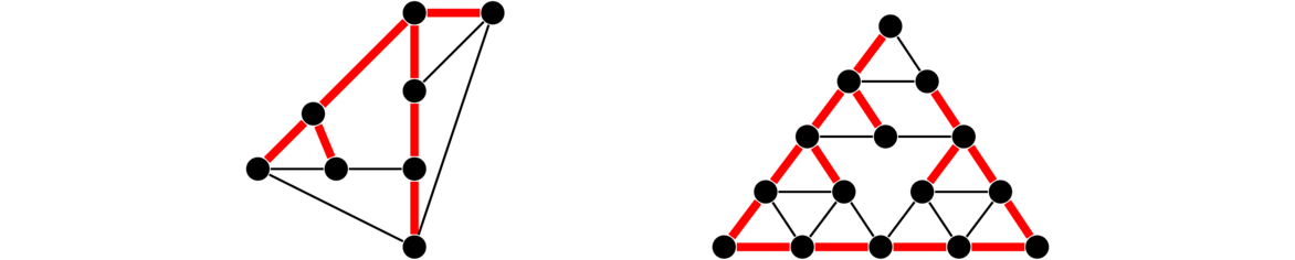
A problem that comes up often is to find a connected subgraph of a graph that uses as few edges as possible. Essentially, we want to be able to get from any vertex to any other, and we want to use as few edges as we can to make this possible. Having a cycle in the subgraph would mean we have a redundant edge, so we don't want any cycles. Thus we are looking for a connected subgraph with no cycles that includes every vertex of the original graph. Such a graph is called a spanning tree. Shown below are two graphs with spanning trees highlighted.

Spanning trees have a number of applications. A nice example shows up in computer network packet routing. Here we have a bunch of computers networked together. Represented as a graph, the computers become vertices and direct connections between two computers correspond to edges. When one computer wants to send a packet of information to another, that packet is transferred between computers on the network until it gets to its destination, in a process called routing. Cycles in that network can cause a packet to bounce around forever. So the computers each run an algorithm designed to find a spanning tree—that is, a subgraph of the network that has no cycles yet still makes it possible to get from any computer to any other computer.

A nice way to find a spanning tree in a graph uses a small variation of the DFS/BFS algorithms we saw earlier. We build up the tree as follows: The first time we see a vertex, we add it to the tree along with the edge to it from the current vertex being searched. If we see the vertex again when searching from another vertex, we don't add the edge that time. Essentially, we walk through the graph and add edges that don't cause cycles until we have reached every vertex. An alternate approach would be to remove edges from the graph until there are no cycles left, making sure to keep the graph connected at all times.

Counting spanning trees

Mathematicians like to count things, and spanning trees are no exception, especially as there is some interesting math involved. In this section, we will use the notation τ(G) to denote the number of spanning trees of a graph G.

One simple fact is that if T is a tree, then τ(T) = 1. Another relatively simple fact is that τ(C_n) = n. This comes from the fact that leaving off any one of the n edges of a cycle creates a different spanning tree, and removing any more than one edge would not leave a tree.

One other fact is that if a graph has a cut vertex, like in the graph below, then the cut vertex essentially separates the graph into two parts, and the spanning trees of the two parts will have no interaction except through that cut vertex. So we can get the total number of spanning trees by multiplying the numbers of spanning trees on either side of the cut vertex, giving 3 × 4 = 12 in total.

One formula for the number of spanning trees relies on something called the contraction of an edge. Contraction is where we essentially “contract” or pinch an edge down to a single point, where the edge is removed and its two endpoints are reduced to a single vertex. Two examples are shown below, where the edge e = uv is contracted into a new vertex w.

Here is the formal definition:

Suppose G is a graph with an edge e = uv. Then the contraction of e in G is an operation that creates a new graph, denoted G · e, that has the same vertices and edges as G except u and v are replaced by a new vertex w which is adjacent to all of the neighbors of u and v in G and nothing else.

Using this, we get the following formula for the number of spanning trees of a graph G:

τ(G) = τ(G-e) + τ(G · e).

Why does this work? First, the spanning trees of G-e are essentially the same as the spanning trees of G that don't include e. Second T(G · e) counts the spanning trees of G that do contain e. This is because any such spanning tree has to include the new double-vertex of G · e, which corresponds to including edge e in the original, since the new double-vertex stands in place of e and its two endpoints.

Here is an example. We will compute the number of spanning trees of G = P₃ □ P₂ as shown below.

Taking the middle edge e out of G leaves us with C₆. Any 5 edges of C₆ (basically leaving out just one edge) make a spanning tree of C₆, so there are 6 spanning trees of C₆. Contracting the middle edge e of G leaves us with the bowtie graph shown above. Any spanning tree must include 2 edges from the left half of the graph and 2 from the right. There are 3 ways to include 2 edges on the left and 3 ways to include 2 on the right, so there are 9 possible spanning trees. So in total in G, we have τ(G) = 6 + 9 = 15.

In general, this spanning tree formula can be recursively applied. That is, we break G into G-e and G · e and then break each of those up further and so on until we get to graphs whose spanning trees we can easily count. For really large graphs, this would get out of hand quickly, as the number of graphs to look at grows exponentially.

Prüfer codes

In this section, we will count the spanning trees of the complete graph K_n. This is the same as the number of ways to connect up n items into a tree. There is a nice technique for this, called Prüfer codes.

We start with a tree with vertices labeled 1 through n. The key step of the Prüfer code process is this:

Take the smallest numbered leaf, remove it, and record the number of its neighbor.

Repeat this step until there are just two vertices left. The result is an (n-2)-tuple of integers. An example of the process is shown below.

Notice that, at each step, the vertex we remove is the one that has the smallest label. We don't record its label in the sequence; instead we record the label of its neighbor. This is what allows us to reconstruct the tree from its sequence.

To do this reconstruction, we do the following: Let P denote the Prüfer sequence, let V denote the sequence of integers from 1 to n, representing the n vertices of the graph. Note that V will always be two elements longer than P. Here is the key step of the reconstruction process:

Choose the smallest integer v of V that is not in P, and choose the first integer p of P. Add an edge between vertices v and p, and remove v and p from their corresponding sequences.

Repeat this step until P is empty. At this point, there will be two integers left in V. Add an edge between their corresponding vertices. An example is shown below, reversing the process of the previous example.

At each step, we take the first thing in P and the smallest thing in V that is not in P. So we won't always be taking the first thing in V.

The Prüfer encoding and decoding processes are inverses of each other. There is a little work that goes into showing this, but we will omit it here. We end up getting a one-to-one correspondence between labeled trees and Prüfer codes. Now each Prüfer code has n-2 entries, each of which can be any integer from 1 through n, so there are n^n-2 possible Prüfer codes and hence that many labeled trees on n vertices. Each of these labeled trees is equivalent to a spanning trees on K_n, so we have τ(K_n) = n^n-2. This result is known as Cayley's theorem.

The Matrix tree theorem

For those who have seen linear algebra, there is a nice technique using matrices to count spanning trees. We start with the adjacency matrix of the graph and replace all entries with their negatives. Then replace all the entries along the diagonal with the degrees of the vertices that correspond to that location in the matrix.

Then delete any row and column and take the determinant. The absolute value of the determinant gives the number of spanning trees of the graph. This remarkable result is called the Matrix tree theorem.

For example, shown below is a graph, followed by its adjacency matrix modified as mentioned above, followed by the matrix obtained by removing the first row and column. Taking the determinant of that matrix gives 15, which is the number of spanning trees in the graph.

Non-isomorphic spanning trees

When we count spanning trees, some of the spanning trees are likely isomorphic to others. For instance, we know that τ(C₆) is 6, but each of those six spanning trees is isomorphic to all of the others, since they are all copies of P₆. A much harder question to answer is how many isomorphism classes of spanning trees are there. For C₆, the answer is 1, but the answer is not known for graphs in general.

Minimum spanning trees

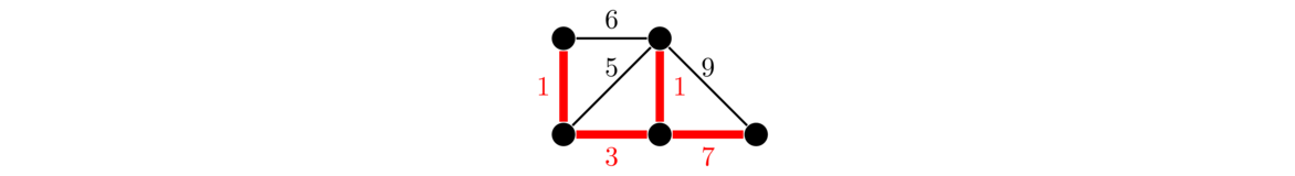
A weighted graph is a graph where we label each edge with a number, called its weight, like shown below.

Weighted graphs are useful for modeling many problems. The weight often represents the “cost” of using that edge. For example, the graph above might represent a road network, where the vertices are cities and the edges are roads that can be built between the cities. The weights could represent the cost of building those roads.

Continuing with this, suppose we want to build just enough roads to make it possible to get from any city to any other, and we want to do so as cheaply as possible. Here is the answer for the graph above:

When solving this problem, since we are trying to do things as cheaply as possible, we don't want any cycles, as that would mean we have a redundant edge. And we want to be able to get to any vertex in the graph, so what we want is a minimum spanning tree, a spanning tree where the sum of all the edge weights in the tree is as small as possible. There are several algorithms for finding minimum spanning trees. We will look at two: Kruskal's algorithm and Prim's algorithm.

Kruskal's algorithm

Kruskal's algorithm builds up a spanning tree of a graph G one edge at a time. The key idea is this:

At each step of the algorithm, we take the edge of G with the smallest weight such that adding that edge into the tree being built does not create a cycle.

We can break edge-weight ties however we want. We continue adding edges according to the rule above until it is no longer possible. In a graph with n vertices, we will always need to add exactly n-1 edges.

An example is shown below. Edges are highlighted in the order they are added.

Kruskal's algorithm is an example of a greedy algorithm. It is called that because at each step it chooses the cheapest available edge without thinking about the future consequences of that choice. It is remarkable that this strategy will always give a minimum spanning tree.

It's worth talking about why Kruskal's algorithm works. We should be sure that the graph T that it builds is actually a spanning tree of the graph. First, T clearly has no cycles because Kruskal's algorithm by definition can't create one. Next, T is connected, since if it weren't, we could add an edge between components of T without causing a cycle. Finally, T is spanning (includes every vertex), since if it weren't, we could add an edge from T to a vertex not in T without causing a cycle. We know that trees on n vertices always have n-1 edges, so we will need to add exactly n-1 edges.

Now let's consider why Kruskal's tree T has minimum weight. Consider some minimum spanning tree S that is not equal to T. As we go through the Kruskal's process and add edges, eventually we add an edge e to T that is not part of S. Suppose we try to add e to S. That would create a cycle by the basic properties of trees. Along that cycle there must be some other edge d that is not in T because T is a tree and it can't contain every edge of that cycle. See below where a hypothetical portion of S is shown along with d and e.

Consider removing d from S and replacing it with e (this is the tree S-d+e). Because we are just exchanging one cycle edge for another, S-d+e is still a spanning tree of G. Now, when the Kruskal's process added edge e, edge d was available to be added (and wouldn't have caused a cycle), but Kruskal's chose e. That means the weight of e is less than or equal to the weight of d. This makes S-d+e is a minimum spanning tree of G that agrees with T on one more edge than S does. We can repeat this process again and again until we get a minimum spanning tree that agrees with T on every edge, meaning that T must be a minimum spanning tree.

It's not too hard to write some code implementing Kruskal's algorithm, though we won't do so here. The trickiest part is checking to see if adding an edge creates a cycle. Something called the disjoint set data structure provides a nice way to do this.

Prim's algorithm

Prim's algorithm is another approach to finding a minimum spanning tree. It is greedy, like Kruskal's, but it differs in how it chooses its edges. Here is how it works: We pick any vertex to start from and choose the cheapest edge incident on that vertex. The tree we are building now has two vertices. Look at all the edges from these two vertices to other vertices, and pick the cheapest one. We have now added three vertices to our tree. Keep this process up, always following the following key rule:

Add the cheapest edge from a vertex already added to one not yet reached.

Just like Kruskal's, we can break edge-weight ties however we like. We stop the algorithm once every vertex has been added to the tree. Here is an example. We will start building the tree from the upper left.

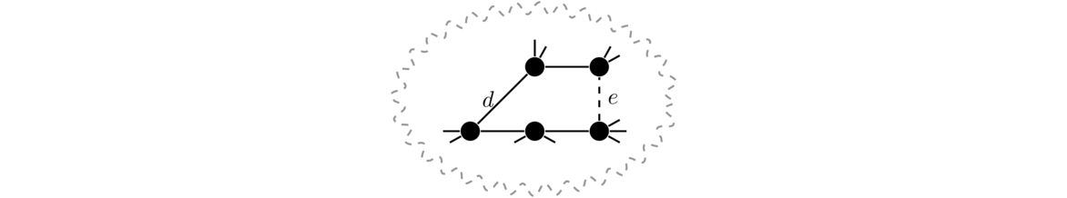
We see that the graph that Prim's algorithm builds up is a tree at every step. This is different from the graph produced by Kruskal's which is disconnected up until the final step. It's interesting to note that Prim's algorithm will not necessarily produce the same tree as Kruskal's. If the edge weights are all different, then the two algorithms will produce the same tree, but if the edge weights are not all different, then there may be multiple minimum spanning trees, and the two algorithms may find different ones.

Though we won't do so, we can show that Prim's algorithm works in a similar way to how we did it for Kruskal's.

A note about greedy algorithms

We referred to Kruskal's and Prim's algorithms as greedy algorithms. A greedy algorithm at each step always chooses the option that looks the best at that step, without consider the consequences of that choice on future steps. For instance, Kruskal's and Prim's algorithms always choose the cheapest edge they can.

This type of strategy doesn't work for all problems. For instance, it would be a pretty bad way to play chess, to only look at the current turn and not consider its effect on future turns. However, greedy algorithms do give the optimal solution to a number of problems in graph theory, and even when they don't, they often give a reasonably good solution quickly.

Shortest paths

In this section we will look at finding the cheapest weighted path between two vertices. Often this is referred to as finding the shortest path in a graph. The most popular method for doing this is called Dijkstra's algorithm. To see how it works, consider the example below in which we are looking for the shortest path from vertex a to vertex g.

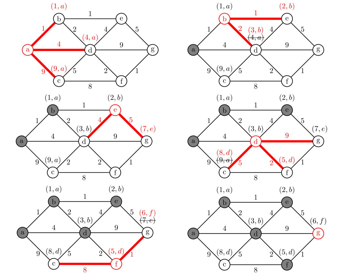
We start from vertex a, visiting each of its neighbors and labeling them with the cost from a, along with an a to indicate that we found them via vertex a. We then mark a as “searched” meaning we will not visit it any more.

We next pick the neighbor of a that was labeled with the smallest cost and visit its neighbors. This is vertex b. Currently, we know that we can get to b from a with a total cost of 1. Since it costs 1 to get from b to e, we label e as (2,b) indicating that we can get from a to e for a total cost of 2 with b indicating that we got to e via vertex b. Similarly, we can get to vertex d with a total cost of 3 by going through b. That vertex d has already been labeled, but our route through b is cheaper, so we will replace the label on d with (3,b). If the cost to d through b had been more expensive, we would not change the label on d. Also, we ignore the edge from b back to a since a has been marked as “searched”. And now that we're done with b, we mark it as “searched”.

We continue this process for the other vertices in the graph. We always choose the next vertex to visit by looking at all the vertices in the graph that have been labeled but not marked as visited, and choose the one that has been labeled with the cheapest total cost, breaking ties arbitrarily. The next vertex to visit would be e, as its total cost is currently 2, cheaper than any other labeled vertex. After a few more steps we get to the point that g is the cheapest labeled vertex. This is our stopping point. Once our goal vertex has the cheapest label, no other route to that goal could possibly be better than what we have. So we stop there, even though we haven't necessarily explored all possible routes to the goal.

We then use the labels to trace the path backward to the start. For instance, at the end g was labeled with (6,f), so we trace backward from g to f. That vertex f was labeled with (5,d), so we trace backward to d and from there back to b and then a, giving us the path abdfg with a total length of 6 as the shortest path.

Algorithm description

Here is a short description of the algorithm in general. Assume the start vertex is called a. The algorithm labels a vertex v with two things: a cost and a vertex. The cost is the current shortest known distance from a, and the vertex is the neighbor of v on the path from a to v that gives that shortest known distance. The algorithm continually improves the cost as it finds better paths to v. Here are the steps of the algorithm:

Start by setting the cost label of each neighbor of a to the cost of the edge from a to it, and set its vertex label to a. Mark a as “searched.” We will not visit it again.
Then pick the labelled vertex v that has the smallest cost, breaking ties however we want. Look at each neighbor of v. If the neighbor is unlabeled, then we label it with a cost of c plus the weight of the edge to it from v. Its vertex label becomes v. If the neighbor is already labeled, we compare its current cost label with c plus the weight of the edge to it the neighbor from v. If this is no better than the neighbor's current cost label, then we do nothing more with this vertex. Otherwise, we update the label's cost with this new cost and update the neighbor's vertex label to v. We repeat this for every unsearched neighbor of v and then label v itself as “searched,” meaning we will not visit it again.
The algorithm continues this way, at each step picking the unsearched labelled vertex that has the smallest cost and updating its neighbors' labels as in Step 2.
The algorithm ends when the labelled vertex with the smallest cost is the destination vertex. That cost is the total cost of the shortest path. We then use the vertex labels to trace back to find the path from the start to the destination. The destination vertex's vertex label is the second-to-last vertex on the path. That vertex's vertex label is the third-to-last vertex on the path, etc.

Dijkstra's algorithm is quite famous and is used in a number of real applications, such as network packet routing.

Eulerian and Hamiltonian graphs

This chapter is about two types of round trips through a graph. The first, called an Eulerian circuit, is a round trip through a graph visiting every edge exactly once; the second, called a Hamiltonian cycle, is a round trip visiting every vertex exactly once. Eulerian circuits turn out to be easy to check for, while Hamiltonian cycles are not.

Eulerian circuits

Traditionally, the first problem in graph theory is considered to be the Brides of Königsberg problem. A sketch of the city of Königsberg and its seven bridges is shown below on the left.

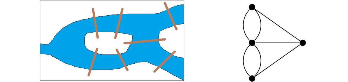
In the early 1700s, some residents wondered if it would be possible to take a round trip through the city that crossed each bridge exactly once. The mayor sent a letter asking about the problem to the famous mathematician Leonhard Euler, who solved the problem by representing it as a graph, essentially inventing the field of graph theory. Euler represented each of the four land regions with a graph, with the bridges corresponding to edges, as shown above on the right.

We can see how the graph retains only the most important information from the map, namely which regions are connected to which other regions via bridges. The exact details of the regions' shapes are not important. By looking at the degrees of the vertices, Euler determined that the desired trip was impossible. The key is the vertices of degree 3. If you start at one of those vertices, you will need to use one of its incident edges to leave that vertex. At some point later, you will use another of its incident edges to arrive back at the vertex and then use the last incident edge to leave the vertex, making it impossible to return to it (remember that we want to finish where we start). If one of those vertices of degree 3 is not the starting point, a similar argument holds, this time leaving us stuck at that vertex with no way to leave after our second visit to that vertex.

We can ask a similar question of any graph: is it possible to walk through the graph, using every edge exactly once and ending up at the start? Such a trip through a graph is named for Euler.

An Eulerian circuit (or Eulerian tour) in a graph is an alternating sequence of vertices and edges in the graph, starting and ending with the same vertex and using each edge exactly once. A graph that has an Eulerian circuit is called Eulerian.

For instance, shown below is an Eulerian circuit in a graph. Edges are labeled in the order they are visited. Notice that every edge is visited, no edge is visited twice, and we end where we start. The graph looks a little busy with all the edges labeled, but to understand how the cycle works, just trace along from edge to edge in the order given.

As in the bridges of Königsburg problem, the key to a graph having an Eulerian circuit is vertices of odd degree (called odd vertices). In particular, if a graph has any odd vertices then it cannot have an Eulerian circuit. What is interesting is that the converse is also true: if a connected graph has no odd vertices, then the graph has an Eulerian circuit. So, other than the obvious part about the graph being connected, the only other thing that can prevent an Eulerian circuit is an odd vertex. Said another way, a graph is Eulerian if and only if every vertex has even degree.

The proof of this is usually done inductively. The basic idea is to pull a cycle off the graph and then combine Eulerian circuits from the left-over pieces into one big circuit using the removed cycle. But what if there is no cycle to pull off? That can't happen, as shown below.

If G is a graph in which every vertex has degree at least 2, then G contains a cycle.

Take a longest path P in G, and consider one of its endpoints v. That vertex is adjacent to a second-to-last vertex on the path, and since v has degree at least 2, there must be another edge incident on it. If that edge's other endpoint is not on the path, we could use it to make a longer path than P. This is impossible, so that edge's other endpoint must be a vertex w of the path. This creates a cycle from v to w and back along the path to v.

This theorem has a variety of uses. Here we use it to prove the theorem about Eulerian circuits. In the proof, we will use the term even graph to refer to a graph in which every vertex degree is even.

A connected graph is Eulerian if and only if every vertex has even degree.

First, if G has an Eulerian circuit, then that circuit must pass into and out of each vertex, perhaps multiple times, adding 2 to its degree count with each pass. Since this circuit accounts for all the edges in the graph, every vertex must have even degree.

We will prove the reverse implication by induction on the number of edges. The base case of 0 edges is trivially true. Suppose the statement holds for all connected even graphs with e edges or less, and consider a connected even graph G with e+1 edges. Since G is connected and even, every vertex has degree at least 2, so by Theorem 10, G has a cycle. Remove the edges of the cycle from G. Every vertex degree in the reduced graph will still be even since we are removing exactly 2 edges from each vertex of the cycle. By the induction hypothesis, each of the components of the reduced graph has an Eulerian circuit. These circuits can be combined with the cycle to create an Eulerian circuit in the original graph by tracing around the cycle such that whenever we reach a vertex that is part of a nontrivial component of the reduced graph, we detour along the Eulerian circuit of that component, returning back to the vertex on the cycle.

An example of the technique in the theorem is shown below. We locate a cycle, in this case abcdef, and remove it. This breaks the graph into several components, each of which has an Eulerian circuit.

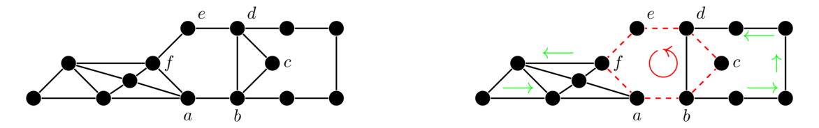
To get an Eulerian circuit of the whole graph, we start by tracing through the cycle from a to b. Next we follow the Eulerian circuit we know exists on the right component of the graph, starting and ending at b. Next we trace along the cycle from c to d to e to f. At f we follow the Eulerian circuit we know exists on the left component of the graph, starting and ending at f. Finally, we go back along the cycle from f to a, completing an Eulerian circuit of the whole graph.

Note here how the induction proof works. We assume that we can handle small cases and use those to build up to bigger cases. Most of the work comes in describing how to use the smaller cases to get the bigger cases. In this case, the trick was to travel along a cycle and detour along the smaller Eulerian circuits.

Finding Eulerian circuits

A simple way to find Eulerian circuits is Fleury's algorithm. Here is how it works:

Start anywhere. At each vertex we choose an edge to add to the tour and then remove it from the graph. We can choose that edge however we like, provided that we never choose a cut edge if there is a non-cut edge available. Taking a cut edge when a non-cut edge is available would cut off part of the graph preventing us from ever reaching it.

For example, in the graph below, suppose we start at vertex a and take the edge to b and from there the edge to d. We would not want to go from d to e as de is now a cut edge and it would prevent us from getting to the right portion of the graph.

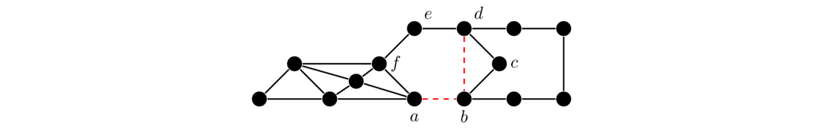
Algorithmically, the only trick to implementing Fleury's algorithm is determining if an edge is a cut edge. We will not include the code here, but it is a nice exercise to try to program it.

Fleury's algorithm is simple, but having to check each edge to see if it is a cut edge makes it somewhat slow. There is another algorithm, called Hierholzer's algorithm, which is more efficient. It is based on the ideas in the induction proof.

Here is how it works: We pick any starting vertex. From that vertex, we walk from vertex to vertex however we like, as long as we don't repeat any edges. We keep track of which edges are used and stop when we end up back at the starting vertex. If all edges of the graph are used, then we're done. Otherwise, we pick any vertex that was part of the first tour that has some unused edges incident on it, and walk from vertex to vertex just like before, taking only unused edges, until we end up back at that new starting vertex. We combine this tour with the first one in the same way described in the induction proof. Then we look for another vertex that is part of the combined tour that still has unused edges incident on it, repeat the previous step, and continue doing this until are the edges are used.

Below is an example.

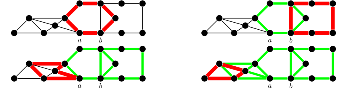
At the first step, we start at vertex a and walk around the middle hexagon to get back to a. There are many other ways we could have walked through the graph to get back to a; it doesn't matter exactly which one we choose. At the next step, we pick a vertex, b, along that walk from a to itself, that has an unused edge incident on it. We do a similar walk starting at b. We add the cycle obtained to our tour by going from a to b, then following the new cycle back to b, and then tracing around the hexagon back to b. We do a similar thing for the remaining two steps.

Cycle decompositions

Even graphs have another interesting property. It is possible to decompose every even graph into cycles. That is, we can find a list of cycles in the graph such that each edge is part of exactly one of them. An example is shown below.

The decomposition consists of a C₃, a C₄, and a C₆. Notice that the cycle edges don't overlap and that every edge is used. Notice also why we need every vertex to have even degree in order to find a cycle decomposition—each cycle contributes a degree of two to each of its vertices. In fact, we have the following theorem.

A connected graph can be decomposed into cycles if and only if every vertex has even degree.

The proof is very similar to the proof for Eulerian circuits, using induction on the number of edges. We locate a cycle in the graph, remove its edges, and note that doing so decreases all vertex degrees of the cycle by 2, leaving them all still even. Thus we have a smaller even graph, which must be decomposable into cycles by the induction hypothesis.

Another way to think of this is we can just keep pulling off cycles until all the edges are used up. When we pull off a cycle, the degrees stay even, so we know there must still be a cycle until only isolated vertices remain.

Notice the similarity this result has with the induction proof of the Euler circuit theorem and with Hierholzer's algorithm.

Eulerian trails

Suppose we remove the restriction from Eulerian circuits about returning back to our starting point. Then we have what is called an Eulerian trail.

An Eulerian trail in a graph is an alternating sequence of vertices and edges in the graph, using each edge exactly once.

By removing the restriction about ending up back at the starting point, we can relax the even vertex condition a bit. Namely, we are now allowed two odd vertices. Try to find an Eulerian trail in the graph below starting at a and ending at b. Notice that a and b are the only odd vertices in the graph.

Remember that what limits an Eulerian circuit to having all even vertices is that whenever we enter a vertex via an edge, we need another edge to be able to exit that vertex. But with an Eulerian trail, we don't need to return the start vertex, nor do we need to leave the end vertex when the trail is done, so those two vertices can have odd degree. But no other ones can. This is stated in the theorem below. Note that the proof relies on a slightly different idea than the discussion here.

A connected graph has an Eulerian trail if and only if no more than two of its vertices have odd degree.

Consider the cases of 0, 1, or 2 vertices of odd degree. If no vertices have odd degree, then they all have even degree, meaning the graph has an Eulerian circuit and hence also an Eulerian trail. Next, by the Handshaking lemma, it's not possible for a graph to have just one vertex of odd degree. Now suppose the graph has two vertices of odd degree. Create a new vertex v adjacent to both of those vertices. The degrees of all the vertices in this new graph are even; hence it has an Eulerian circuit. The portion of the circuit excluding v is an Eulerian trail in the original.

Now we prove the converse. Suppose the graph has an Eulerian trail. If the two endpoints of the trail are adjacent, then we can use the edge(s) between them to create an Eulerian circuit. Since the graph has an Eulerian circuit, all the vertices in the graph have even degree. On the other hand, if the two endpoints are not adjacent, add a new vertex v that is adjacent to both of the endpoints. If we take the trail along with the two edges into v, we have an Eulerian circuit in the new graph. Hence the degree of every vertex in the new graph must be even. This means that all the vertices in the original graph must have an even degree except for the two endpoints of the trail.

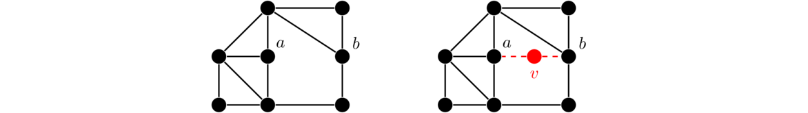
Above is a picture of what is going on in the proof. In the picture there are two vertices a and b of odd degree. In the first part of the proof, we add the vertex v adjacent to a and b to make the graph even. The new graph has an Eulerian circuit, so that circuit minus the two new edges is an Eulerian trail in the original. For the second part of the proof, trace through the graph to find an Eulerian trail starting at a and ending at b. Adding the new vertex creates an Eulerian circuit, which means all the vertices in the new graph have even degree; thus all the vertices of the original have even degree except for a and b.

Applications

Eulerian trails and circuits have applications to a number of problems. For instance, they apply to planning routes for street sweepers, snow plows, and delivery people. There is a more general problem, called the Chinese postman problem, where we want to visit every edge in a graph and do so as efficiently as possible. The edges might have weights indicating the costs to take them, and some edges might have to be repeated. To solve this problem, the graph is modified into another graph, and an Eulerian circuit in the modified graph is used to solve the original problem.

Eulerian circuits can also be used to find De Bruijn sequences, which are sequences of numbers with special properties that make them useful for everything from card tricks to experiment design.

Eulerian circuits can also be used in reconstructing DNA from fragments and in CMOS circuit design.

Hamiltonian cycles

In this section, instead of visiting every edge of a graph exactly once, we want to visit every vertex exactly once, returning to our starting point. This is called a Hamiltonian cycle.

A Hamiltonian cycle in a graph is a subgraph that is a cycle and includes all the vertices in the graph. A graph that has a Hamiltonian cycle is called Hamiltonian. A Hamiltonian path is a subgraph that is a path including all the vertices in the graph.

They are named for William Rowan Hamilton, best known for his work in physics and quaternions, who once tried marketing a board game based on Hamiltonian cycles. Below are a few graphs with Hamiltonian cycles highlighted.

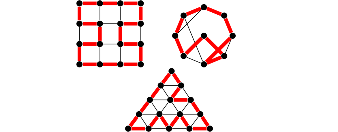
Just to reiterate: we want to visit each vertex exactly once and end up back where we started. Some edges might not be used.

Unlike with Eulerian circuits, there is no easy answer to whether a graph contains a Hamiltonian cycle. And even if we know a graph must have a Hamiltonian cycle, that doesn't mean the cycle is easy to find. For Eulerian circuits, we had a necessary and sufficient condition—no odd-degree vertices—that we could use to tell whether or not a graph was Eulerian. With Hamiltonian cycles, there are some relatively simple necessary conditions and some relatively simple sufficient conditions, but we don't have anything simple and useful that works both ways. In fact, finding a simple and fast check that works for all graphs is literally a million-dollar problem, equivalent to the famous P = NP problem.

Showing a graph doesn't have a Hamiltonian cycle

If a graph contains a cut vertex or a cut edge, then clearly the graph has no Hamiltonian cycle as once we cross that cut vertex/edge, there is no way to get back across to complete the cycle. In the graph below, we see there is no way to get back to the other side of the graph when we cross over either a or edge bc.

Here is a useful generalization of the cut vertex/edge idea.

If there is some subset S of vertices of G such G-S has more components than S has vertices, then G has no Hamiltonian cycle.

For instance, we can try to remove 1 vertex that breaks the graph into 2 or more components. This would be a cut vertex. Or we can try to remove 2 vertices to break the graph into 3 or more components. Or we could try to remove 3 vertices to break the graph into 4 or more components, etc. Below is an example. We'll take S = {a,b}. The three components of G-S are shown on the right.

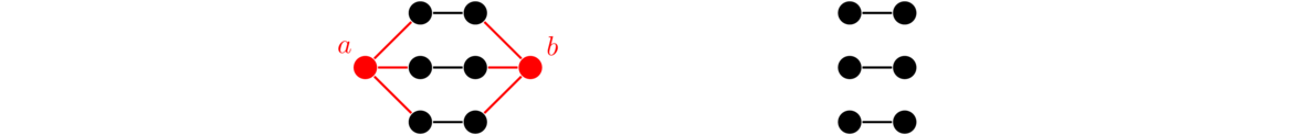
The number of components of G-S is greater than |S|, so there is no Hamiltonian cycle. Essentially what happens is a and b act as a bottleneck. Any time we want to leave one of the components of G-S, we have to use either a or b. We use up a and b this way and can't complete our round trip.

The theorem is often stated in a more positive way, like this: If G has a Hamiltonian cycle, then for every subset S of vertices, the number of components of G-S is less than or equal to |S|. Our version is the contrapositive of this. However, the positive version is a little easier to prove. The basic idea is as we trace through a Hamiltonian cycle in G, any time we reach a component of G-S, the only way to reach other vertices not in that component is by going back through S. Thus, S must have at least as many vertices there are components of G-S. The figure below might be helpful in understanding the proof.

Another example is below. Four vertices are deleted and the resulting graph has five components, so there is no Hamiltonian cycle.

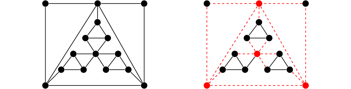
Note that this theorem provides a necessary, but not sufficient, condition for a Hamiltonian cycle. There are many graphs that pass this condition that don't have Hamiltonian cycles. The Petersen graph is one such example. There are other necessary conditions for Hamiltonian cycles besides this one, though we won't cover them here.

Showing a graph has a Hamiltonian cycle

There are quite a number of theorems that guarantee a graph has a Hamiltonian cycle provided the graph has certain properties. One of the simplest ones is Dirac's condition.

Dirac's condition

(Dirac's condition) In a simple graph with n ≥ 3 vertices, if every vertex is has degree at least n/2, then the graph has a Hamiltonian cycle.

Find a maximum length path P in the graph. Let its vertices be called v₁, v₂, …, v_k. We will show that P can be made into a cycle C. If v₁ and v_k are adjacent, then clearly we have a cycle. Otherwise, we will find a cycle by showing that there are two adjacent vertices on the path, v_i and v_i+1, with v₁ adjacent to v_i+1 and v_k adjacent to v_i. We would then have the cycle v₁, v₂, …, v_i, v_k, v_k-1, … v_i+1, v₁, as shown below.

To see why these vertices v_i and v_i+1 must exist, first note that the endpoints v₁ and v_k can have no neighbors that are not on P as otherwise we could extend the path to a longer one. So v₁ is adjacent to at least n/2 of the vertices from v₂ through v_k-1. We just need v_k to be adjacent to a vertex on the path immediately preceding one of these n/2 vertices. If somehow it wasn't, then there would be n/2 vertices on the path that v_k was not adjacent to, which is impossible since v_k has at least n/2 neighbors and they all must lie on the path.

Finally, we must show that the cycle C just found actually contains every vertex of the graph. Suppose there were some other vertex w not on C. Since v₁ is adjacent to n/2 vertices, all of which are on P, more than half of the graph's vertices are on P. Therefore, since deg(w) ≥ n/2, w must be adjacent to some vertex v_j of P. But then we could create a longer path than P by starting at the vertex immediately after v_j on the cycle C, tracing back around to v_j and then detouring out to w. This is impossible, so every vertex of the graph must lie on C, making C a Hamiltonian cycle.

It's worth pausing here to realize what we have done: We have shown that for any graph at all, as long every vertex is adjacent to at least half of the vertices, then that graph has a Hamiltonian cycle. The proof is what is called an “existence proof” in that it shows that there is a Hamiltonian cycle, but it doesn't really show how to find it. The first step of the proof, finding a longest path, turns out to be as hard as finding a Hamiltonian cycle.

This condition that every vertex be adjacent to at least n/2 vertices guarantees that each vertex has a pretty high degree, giving the graph a lot of edges and giving us a lot of freedom to try to create a Hamiltonian cycle. Note that the n/2 of the theorem cannot be reduced any further. For instance, in the graph below, every vertex has degree at least n/2-1, but there is no Hamiltonian cycle due to the cut vertex.

Ore's condition

The condition above is known as Dirac's condition for the graph theorist Gabriel Dirac who discovered it in 1952. A few years later Øystein Ore noticed that it isn't necessary that every single vertex have degree at least n/2. Rather it is enough that the degrees of any pair of nonadjacent vertices must add up to at least n.

(Ore's condition) In a simple graph with n ≥ 3 vertices, if for every pair of nonadjacent vertices u, v in the graph we have deg(u)+deg(v) ≥ n, then the graph has a Hamiltonian cycle.

The proof works almost the exact same way as the proof of Dirac's condition (and it is a good exercise to try it). Most likely, Ore had carefully read through the proof of Dirac's condition and noticed that the proof would still work even if not every vertex had degree n/2. He probably thought about how he could modify the hypothesis and still have the proof work.

Notice that if a graph satisfies Dirac's condition then it also satisfies Ore's condition, since if every vertex has degree n/2, then for any pair of nonadjacent vertices u and v (or even for adjacent vertices), we have deg(u)+deg(v) ≥ n/2+n/2 = n. Ore's condition is a weaker condition than Dirac's. It applies to more graphs than Dirac's condition, though it is a little trickier to use.

To test it, look at all pairs of nonadjacent vertices and make sure in every such case their degrees sum up to at least n. For example, in the graph below on the left, each vertex has degree 3 or 5. There are some degree 5 vertices that are not adjacent to each other, but their degrees sum to 10, which is greater than n = 8. The degree 3 vertices are not adjacent to some degree 5 vertices, but in this case the degrees sum to 3+5 = 8, so this is okay. So the left graph passes Ore's condition and thus has a Hamiltonian cycle.

On the other hand, the graph on the right fails Ore's condition because the two degree 3 vertices are not adjacent, and their degrees sum to 3+3 = 6, which is not at least 8. So Ore's condition cannot be used to show the graph has a Hamiltonian cycle. Nevertheless, the graph does have one. This demonstrates a weakness of purely sufficient conditions: they miss some graphs that do have Hamiltonian cycles.

The Bondy-Chvátal condition

Building on Ore's condition, J.A. Bondy and Václav Chvátal found that adding an edge between nonadjacent vertices whose degrees add up to at least n has no effect on whether or not a graph has a Hamiltonian cycle.

To see why, take a graph G with no Hamiltonian cycle and add an edge between nonadjacent vertices u and v whose degrees add up to at least n. Suppose that G+uv actually has a Hamiltonian cycle. In that case, the cycle minus edge uv would be a path from u to v containing every vertex of G (a Hamiltonian path). By the same ideas as in the proof of the Dirac/Ore conditions, we can create a Hamiltonian cycle involving this path. But this is impossible as G has no Hamiltonian cycle. Hence G+uv can't have one either.

This leads to the following process: Find a pair of nonadjacent vertices whose degrees add up to at least n, add an edge between them, and keep doing so for other such pairs of vertices in the graph. As we add edges, this will increase the degrees of vertices, possibly creating new pairs of nonadjacent vertices whose degrees now add up to at least n. This is okay, and we add edges to make them adjacent as well. We continue this until it is no longer possible.

The graph we obtain through this process is called the closure. It is interesting to note that the closure is unique—no matter what order we add edges, in the end we will always end up at the same graph. We have the following theorem:

(Bondy and Chvátal's condition) A graph is Hamiltonian if and only if its closure is Hamiltonian.

Thus Bondy and Chvátal's condition gives us a way to check for Hamiltonian cycles. Add edges as described above to find the closure and then see if the closure has a Hamiltonian cycle. The closure will hopefully have quite a few more edges, making it easier to spot a Hamiltonian cycle in the closure than in the original. Here is an example. On the left is a graph and on the right is its closure.

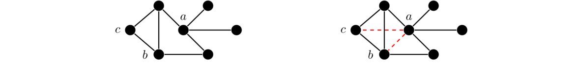
The graph has 7 vertices, and initially vertex a has degree 4 and b has degree 3. Since deg(a)+deg(b) = 7, we can connect a and b. After doing that, a now has degree 5, so now we have deg(a)+deg(c) = 7, so we can connect a and c. However, this is as far as we can go.

So the closure of this graph consists of the original graph along with the new edges ab and ac. It is pretty clear from the start that the graph has no Hamiltonian cycle, and notice that the closure, despite the added edges, still has no Hamiltonian cycle.

Here is another example. On the left is a graph and on the right is its closure.

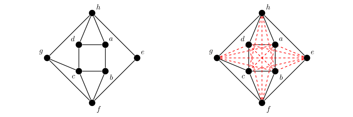
To find the closure, first note that there are 8 vertices, so we are looking to add edges between nonadjacent vertices whose degrees add up to at least 8. Vertices f and h are not adjacent and their degrees add up to 8, so we can add edge fh. This brings the degrees of f and h up to 5. Each vertex on the center square has degree at least 3, so their degrees when added to the new degrees of f and h will be at least 8, so we can add edges from every vertex on that square to whichever of f and h they are not adjacent to. This brings the degrees of all the vertices on the square up to at least 4, so now we can add edges ac and bd.

This brings the degrees of vertices a, b, and d up to 5, and as g has degree 3, we can add edges from g to each of them. Now every vertex in the graph has degree at least 6 except for e, which has degree 2. But as 6+2 = 8, we can add edges from e to every other vertex. So in the end, the closure ends up being the complete graph K₈, which clearly has a Hamiltonian cycle. Thus by the Bondy-Chvátal condition, the original graph must have a Hamiltonian cycle as well.

Notice, unfortunately, that the Bondy-Chvátal condition tells us that there is a Hamiltonian cycle in the original, but it doesn't tell us how to actually find that cycle.

Pósa's condition

In 1962, Lajos Pósa gave a different set of conditions for a graph to be Hamiltonian.

(Pósa's condition) Let G be a graph with n ≥ 3 vertices where the degrees are d₁ ≤ d₂ ≤ … ≤ d_n. If d_i > i holds for i < n/2, then G is Hamiltonian.

This can be proved in a straightforward way from the other conditions, though we won't do so here. The d₁ ≤ d₂ ≤ … ≤ d_n part just says to arrange the degrees in order. The d_i > i part says that we have to check that d₁ > 1, d₂ > 2, d₃ > 3, etc., and the i < n/2 part says that we don't need to check all the vertices, just one less than the first half of the vertices.

For example, consider the graph below on the left. We first put the vertices in order by degree, which gives us degrees 2, 3, 3, 3, 3, 4, 4, 4. There are 8 vertices, and 8/2-1 = 3, so we just have to check the first 3 degrees, namely that d₁ > 1, d₂ > 2, and d₃ > 3. The first two work since 2 > 1 and 3 > 2, but the third one fails since 3 ≯ 3. So Pósa's condition cannot be used to tell us if this graph has a Hamiltonian cycle.

As another example, consider the graph above on the right. Putting the vertex degrees in order gives 2, 3, 4, 5, 5, 5, 5, 6, 6, 7. There are 10 vertices, and 10/2-1 = 4, so we have to check the first 4 degrees. Doing so gives 2 > 1, 3 > 2, 4 > 3, and 5 > 4. All of these check out, so Pósa's condition tells us there is a Hamiltonian cycle in this graph.

It might seem strange that we only have to check 4 of the 10 vertices in the graph, but the fact that we've put things in numerical order means that all of the other vertices must have a reasonably high degree, namely at least 5 in this case and n/2 in general.

Chvátal's condition

Chvátal took Pósa's condition one step further. He said that it is okay, for instance, for some of Pósa's inequalities to fail, but only as long as that is compensated by there being other high degree vertices in the graph.

(Chvátal's condition) Let G be a graph with n ≥ 3 vertices where the degrees are d₁ ≤ d₂ ≤ … ≤ d_n. If for each i < n/2 we have either d_i > i or d_n-i ≥ n-i, then G is Hamiltonian.

For example, consider the graph below. In order, its 10 degrees are 2, 2, 4, 5, 5, 6, 7, 8, 8, 8. Since there are 10 vertices, we have n/2-1 = 4, so we have to check the condition for i = 1, 2, 3, and 4.

For i = 1, we have d₁ = 2, so d₁ > 1 and that's good. For i = 2, we have d₂ = 2 and 2 ≯ 2, so this graph would fail Pósa's condition. However, Chvátal's condition gives us a way out. For i = 2, it says we either need d₂ > 2 or d₈ ≥ 8. Since d₈ = 8, we are good there. Next, for i = 3, it says we need d₃ > 3 or d₇ ≥ 7. We have d₃ = 4, so this case is taken care of. Finally, for i = 4, we need d₄ > 4 or d₆ ≥ 5. We have d₄ = 5, so that's good. All four cases check out, so the graph has a Hamiltonian cycle.

Other conditions

It is important to note that all of the conditions from Dirac's through Chvátal's are sufficient, but not necessary. For example, C₁₂ fails every one of these conditions yet still has a Hamiltonian cycle.

There are many other sufficient conditions besides these, many of which apply to only to particular kinds of graphs. For instance, if a graph is regular and each vertex is adjacent to at least one third of the vertices in the graph, then the graph has a Hamiltonian cycle. Finding sufficient conditions like this is still an active area of research.

The Traveling Salesman Problem and NP Completeness

The Traveling salesman problem

Hamiltonian cycles are related to the famous Traveling salesman problem. In that problem, a salesman needs to visit several cities in a row and return home. There are various costs associated with traveling from one city to another, and the salesman wants to book the cheapest trip possible that covers all the cities. As a graph problem, the cities are vertices, an edge between vertices indicates it is possible to go directly between their two cities, and weights on the edges correspond to the cost of traveling between the two corresponding cities. We are looking for a minimum weight Hamiltonian cycle. For example, shown below is a graph with an optimal solution highlighted.

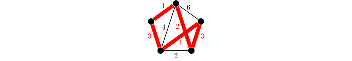
This problem has been extensively studied by mathematicians and computer scientists. The brute-force way to find a solution is to check every possible route, but if every city is connected to every other one, then there are n! possible routes, which gets out of hand very quickly. Some clever techniques, such as dynamic programming, can bring the number of routes to check down to n²2ⁿ, a considerable improvement, but still exponential. Despite this, people have been able to find algorithms that work for maps consisting of many thousands of cities. There are also many approximate algorithms that don't find an exact solution but do find one that is guaranteed to be within a certain percentage of the optimal answer.

NP completeness

We have seen a number of graph algorithms so far. One of the most important considerations is how quickly they run. In particular, as we increase the number of vertices and/or edges in a graph, how does that affect how long it takes the algorithms to run.

Running times

Here is a little introduction to how running times of algorithms are typically measured. Suppose we have the following Python code that adds up all the values in a list:

total = 0
for i in range(len(L)):
    total += L[i]

Suppose the list has n items. The code looks at each item and takes a certain amount of time to add its value into the total. It also takes a certain amount of time to do other little things, like setting the total to 0. So the running time of this algorithm on a particular computer might be something like 2.3n + .2 microseconds. The constants 2.3 and .2 will vary from computer to computer. We don't actually care about them. All we care about is the n. This is usually written as O(n), which is read as “big O of n”. It tells us the order of growth of the running time.

Since the order of growth is O(n), this is a linear algorithm, meaning if we double the amount of items in the list, the running time will roughly double. If we triple the amount of items, the running time will roughly triple.

As another example, suppose we want to add up the items in an n × n matrix. In this case, the running time might be something like 3.4n²+.2. We would write this as O(n²). This tells us that the running time grows as the square of n. This is a quadratic algorithm. In particular, if we double the number of entries, then the running time would more or less quadruple. If we triple the number of entries, the running time would go up by a factor of about 9.

Both of these are examples of polynomial growth. Any algorithm whose running time is a polynomial is called a polynomial-time algorithm. A capital P is used to denote the collection of all algorithms that run in polynomial time.

Not all algorithms run in polynomial time. For example, if we were to list out all the subsets of {1,2,…,n}, that would be an O(2ⁿ) algorithm, as there are 2ⁿ subsets. This is an example of an exponential algorithm. Here, just adding one more element to the set will double the running time.

Polynomial-time algorithms are generally preferred to exponential-time algorithms. To see why, consider the huge differences in growth between n² and 2ⁿ shown below:

10² = 100
2¹⁰ = 1024
100² = 10,000
2¹⁰⁰ = 1.27 × 10³⁰
1000² = 1,000,000
2¹⁰⁰⁰ = 1.07 × 10³⁰¹

For example, suppose we had to choose from two algorithms to do something on a graph, one of which was O(n²) and the other was O(2ⁿ). On a graph with 1000 vertices, the table tells us the O(n²) algorithm would have a running time on the order of about 1,000,000 time units. If those time units are microseconds, then the algorithm takes around a second to run. On the other hand the O(2ⁿ) algorithm takes 1.07 × 10³⁰¹ time units, which is far, far greater than the age of the universe. In practical terms, the exponential algorithm is unusable.

Note that exponential algorithms can sometimes outperform polynomial algorithms if the number of vertices is relatively small. We will leave out the details here. They idea is that eventually, once the number of vertices gets large enough, exponential algorithms are far worse than polynomial algorithms.

The NP collection of problems

There is another collection of problems, denoted NP, where if we are given a solution to them, it takes a polynomial amount of time to check that the solution indeed works. To find a solution may or may not take a polynomial amount of time, but to check that a solution works must take polynomial time if an algorithm is to be in NP.

Anything that is in P is also in NP, but NP contains some other problems that are thought not to be in P. One example is Sudoku. Given a solution to a Sudoku, it's not too hard to check that is works. We just have to run through each row, column, and block, making sure there are no repeats. However, solving Sudokus is quite a bit more challenging. No one knows a polynomial algorithm that finds solutions to n × n Sudokus.

Here is another example, called the subset sum problem: Given a set of integers, is it possible to find a subset of them summing to exactly 0? For example, given the set {-20,-12,-10,-7,-3,4,5,9,18,25}, try to find a subset whose elements sum to 0. It takes some time and thought to do this; however, it takes very little time or thought to verify that {-12,-10,4,18} works. For a set with thousands of elements, it can take a tremendous amount of time to find a solution, but very little time to add up the elements of a potential solution to check that it works.

Sudoku and the subset sum problem are called NP-complete problems. That is, they are in NP and they are at least as hard as any problem in NP. What this means is that if someone were to find a polynomial-time solution to an NP-complete problem, then they could use that solution to find a polynomial-time solution of any other NP-complete problem. No one has found a polynomial-time solution to an NP-complete problem. The best solutions so far that have been found are exponential-time.

As mentioned earlier, P is contained in NP. The big question, though, is does P equal NP? This is called the P = NP problem, and is one of the most famous unsolved problems in math. It basically asks this:

If we can efficiently check if a solution is correct, does that mean we can efficiently solve the problem?

There is a million-dollar prize for its solution. Most mathematicians and computer scientists think that P is not equal to NP, but not everyone agrees, and no one has come close to solving the problem.

Relation to graph theory

Here is where this relates to graph theory: Some of the problems we have seen are in P. These include Eulerian circuits, shortest paths in graphs, and minimum spanning trees. Other problems we have seen are NP-complete. These include Hamiltonian cycles, longest paths in graphs, and finding maximum independent sets.

When we say that the Eulerian circuit problem is in P, we mean that there is a polynomial algorithm that determines if a graph has an Eulerian circuit or not. Going through and checking the degrees of each vertex to see if they are all even is a polynomial algorithm. Hierholzer's and Fleury's algorithm for finding those circuits are also polynomial algorithms.

On the other hand, the Hamiltonian cycle problem is NP-complete. The problem is in NP because if someone gives us a Hamiltonian cycle in a graph, it is easy (polynomial-time) to check that it really is a Hamiltonian cycle. However, people have proved that a polynomial-time solution to the Hamiltonian cycle problem would provide a polynomial-time solution to any other problem in NP. Thus the Hamiltonian cycle problem is NP-complete. No one has found a polynomial-time solution to the Hamiltonian cycle problem, and it is very likely that no one ever will.

Similarly, Dijkstra's algorithm for shortest paths runs in polynomial time (O(n²) or better, depending on how the algorithm is implemented). On the other hand, finding the longest path in a graph is NP complete. The only known algorithms are exponential-time, which means finding the longest path in a graph can take a long time, especially for large graphs.

In short, if a graph problem turns out to be in P, then there is most likely an algorithm that solves the problem fairly quickly, even for relatively large graphs. On the other hand, if it is NP-complete, then solving the problem for arbitrary large graphs will likely be difficult and take an unmanageable amount of time.

However, sometimes the problem will be manageable on specific classes of graphs. For instance, finding Hamiltonian cycles is an NP-complete problem, which means we don't really expect to have a good algorithm that works for any graph, but if we just restrict ourselves to complete graphs, then the problem is easy. As another example, finding maximum independent sets is an NP-complete problem, but if we just want to find maximum independent sets on trees, that is a manageable (polynomial-time) problem.

Coloring

Definitions and examples

In graph coloring we assign labels (called colors) to the vertices of a graph so that adjacent vertices get different colors. We are usually interested in using as few colors as possible. A little later we will explain where the term “colors” comes from, but for now the colors we assign will be positive integers. Here are a few example colorings of a graph:

The coloring on the left is bad as it assigns the same color to adjacent vertices. The middle coloring is better, as it satisfies the rules, but it uses more colors than are needed. The right coloring is the one we are after. It satisfies the rules and uses as few colors as possible. It wouldn't be possible to use less than three colors as the triangles in the graph require three colors. Here is the formal definition of coloring.

A coloring of a graph is an assignment of labels, called colors, to the vertices of the graph. A proper coloring is a coloring such that adjacent vertices are never assigned the same color. The chromatic number of a graph G, denoted χ(G), is the minimum number of colors needed to properly color a graph.

If it's clear what graph we are referring to, we will abbreviate χ(G) as χ. To understand something new, it often helps to try it on some simple classes of graphs, like paths, cycles, etc., so let's look at them.

Paths

Here are some optimal colorings on paths:

In general, χ(P_n) = 2 for every n ≥ 2.

Cycles

Here things are a little more interesting, as odd and even cycles behave differently. It is not to hard to show that odd cycles always have a chromatic number of 3, while even cycles have a chromatic number of 2.

Complete graphs

Since every vertex is adjacent to every other vertex in a complete graph, we cannot repeat any colors. Thus χ(K_n) = n.

Bipartite graphs

The chromatic number of any bipartite graph is 1 or 2. Some people find this a little tricky, but it's simple once you think about it the right way. A partite set is an independent set, with no edges between its vertices, so we can color all of its vertices the same color. With two partite sets, we thus need two colors. And this applies to any bipartite graph, not just complete ones.

In fact, this result goes both ways: any graph with at least one edge is bipartite if and only if it is 2-colorable. The algorithm of Section 3.1 is essentially an algorithm to two-color a graph. Further, since trees are bipartite, we now know that all nontrivial trees have chromatic number 2.

Unions and joins

We have χ(G ∪ H) = max(χ(G), χ(H)). This is because there are no edges between the copies of G and H in the union, so we can color each graph separately without worrying about its colors affecting the other graph. See below on the left for a coloring of C₄ ∪ C₃.

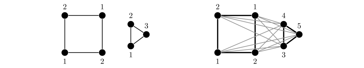
We also have χ(G∨ H) = χ(G)+χ(H). Every vertex of G is adjacent to every vertex of H, so no color used on G can be used on H and vice-versa. To get a proper coloring of G∨ H, we can color G and H separately and then replace each color c of H with c+χ(G), basically shifting the colors. A coloring of C₄ ∨ C₃ is shown above on the right.

Cartesian product

The Cartesian product is a little trickier. The result is χ(G □ H) = max(χ(G), χ(H)), which is the same as for the union. This might be a little surprising since there are so many more connections in the Cartesian product than in the union.

Let's look at an example: C₅ □ C₄. Highlighted below is a particular vertex.

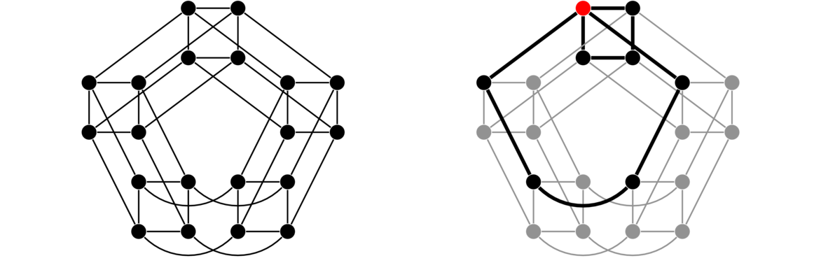
The highlighted vertex is essentially a part of two graphs at once: C₅ and C₄. We need to make sure its coloring works with respect to both graphs. We can think of C₅ □ C₄ as consisting of five copies of C₄ with the connections between copies determined by the connections of C₅. Our approach will be to color each of the five copies of C₄ in its own way, making sure that the interactions between the copies (which are determined by C₅) are respected.

We start with the optimal colorings below of C₄ and C₅.

The trick is for each vertex to take its color in C₄, its color in C₅, and add them, reducing the result modulo 3, replacing any zeros obtained with threes (though this replacement is not strictly needed). The colorings for the five copies end up looking like this:

Doing things this way guarantees that adjacent vertices will never get the same color. Its a nice exercise to try to prove why. The same process works in general. For graphs G and H, let m = max(χ(G), χ(H)) and color a vertex (u,v) of G □ H with the color (c_G(u)+c_H(v)) mod m, where c_G(u) and c_H(v) are its colors in G and H, respectively.

An arbitrary graph

Here is one more example, this one a graph with no obvious structure. Try coloring it before looking at the answer to the right.

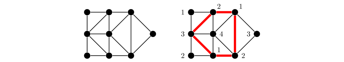
Without any obvious structure it can take some effort to come up with an answer. There are lots of triangles in the graph, so we will need to use at least 3 colors, but will we need more? The answer is yes. Highlighted in the graph on the right is a 5-cycle. It requires 3 colors. The vertex in the middle of that cycle is adjacent to the entire cycle, so we can't reuse any of the cycle's colors on it. Thus 4 colors are required.

Properties

Lower bounds

When trying to color graphs, one of the first things to notice is that if the graph contains a triangle (a C₃ or K₃ subgraph), then the graph will need at least three colors. This is because all three vertices in a triangle are adjacent and therefore must get different colors. This generalizes to larger cliques (complete subgraphs).

For any graph whose largest clique is of size ω, we have χ ≥ ω.

The proof is a nice exercise. In fact, generally, if H is any subgraph of G, then χ(G) ≥ χ(H). Here is another lower bound for the chromatic number.

For any graph on n vertices whose largest independent set is of size α, we have χ ≥ n/α.

All the vertices with a given color form an independent set, called a color class. If we add up the sizes of all the color classes, we get n, the total number of vertices in the graph. Each color class has at most α vertices and there are χ color classes, so the sum of the sizes of the color classes is at least as large as χ · α. Thus χ · α ≥ n. Divide both sides by α to conclude the proof.

For an example of this theorem, consider the graph below.

Let's see how large of an independent set we can find. The vertices x, y, and z form a triangle, so at most one of them can be part of an independent set. Looking at the other four vertices, the only independent set with two vertices is {a,c}, but taking both of those would conflict with whatever vertex we took from triangle xyz. Thus for this graph, α = 2. Then by the theorem, we have χ ≥ n/α, so χ ≥ 7/2, which is 3.5. But χ is an integer, so we need at least 4 colors for this graph. A 4-coloring is shown on the right above.

Note

For a graph G, the constants ω and α, that we saw in the theorems above, are important in many contexts besides graph coloring. They are known as the clique number and the independence number of the graph.

Greedy coloring

A natural question is if there is a good algorithm for coloring graphs. If we want an algorithm that runs quickly and gives the exact value, that is quite possibly hopeless, as graph coloring is NP-complete. On the other hand, the following algorithm, called the greedy algorithm, is very quick and reasonably good. Here is how it works:

First, decide on an order in which to visit the vertices. Then visit the vertices in that order, assigning each vertex the smallest color available that hasn't already been used on one of its neighbors.

Here is an example. In the graph below, let's order the vertices in counterclockwise order starting at the lower right. The ordering is indicated by the circled numbers.

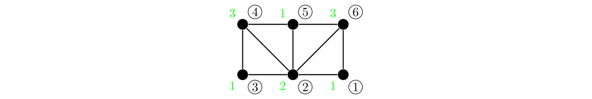
To color the graph, we can use color 1 on vertex 1. Then color 1 is not available on vertex 2, so we color it with 2. On vertex 3, color 1 is available, so we use it there. Vertex 4 has neighbors colored 1 and 2, so we must use color 3 there. Color 1 is again available on vertex 5, but on vertex 6 we are stuck using color 3 again.

The “greedy” part of this algorithm is that it always chooses the smallest coloring currently available without any thought to the consequences of that choice. Unlike with greedy algorithms for spanning trees, where greedy algorithms always find the optimal answer, greedy coloring usually does not find the optimal answer. In fact, on average, for a large random graph with a randomly chosen ordering, the greedy algorithm will use on the order of about twice as many colors as the minimum. Below on the left is a graph and an ordering that uses more colors than necessary.

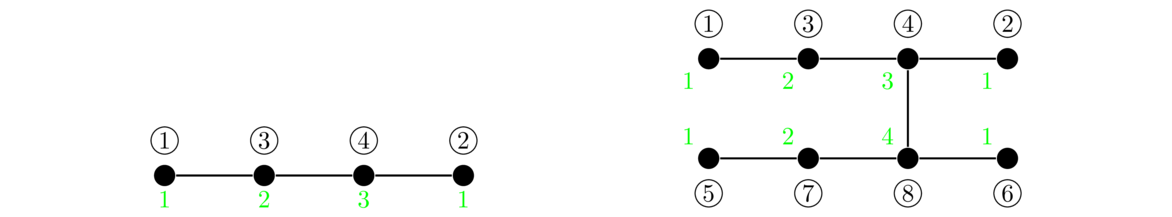
On the right is another graph that requires only two colors along with an ordering that forces the greedy algorithm to use 4 colors. It's possible to extend these examples into bipartite graphs (2-colorable) with orderings that force a huge number of colors.

It's interesting to note that there is always some ordering for which the greedy algorithm will give an optimal coloring, though finding that ordering is as difficult as finding the chromatic number.

Upper bounds

One immediate consequence of the greedy algorithm is that χ ≤ Δ+1, where Δ is the largest vertex degree in the graph. This is because at any stage of the algorithm, no vertex will have any more than Δ previously colored neighbors, so we won't need more than Δ+1 colors. If we work a bit harder, we can reduce this by 1 most of the time. This result is called Brooks' theorem. It is stated below, but we won't prove it, as the proof is a bit involved.

(Brooks' theorem) For any graph, χ ≤ Δ+1. If it is not complete or an odd cycle, then χ ≤ Δ.

For example, the graph below is not a complete graph, not an odd cycle, and its maximum degree is 4. Thus, we know we will not need more than 4 colors. Further, its maximum clique is of size 3, so we will need at least 3 colors. Thus combining upper and lower bounds, we know that this graph can be colored in either 3 or 4 colors.

Note that the other lower bound, χ ≥ n/α is not of much help here. There are 8 vertices and an independent set of size 4, so it just tells us that χ ≥ 2.

A little more about the greedy algorithm

A useful strategy for greedy coloring is to put the high degree vertices early in the ordering. In particular, let the vertices of a graph be v₁, v₂, …, v_n, arranged by degree such that deg(v₁) ≤ deg(v₂) ≤ deg(v_n). Visit the vertices in the order of v_n, v_n-1, … v₁. In the worst case scenario, v_n gets color 1, v_n-1 gets color 2, etc., but eventually we get to some vertex whose color exceeds its degree. At that point, we know we don't need to introduce any new colors.

Mycielski's construction

We know that if a graph contains a triangle, then it its chromatic number is at least 3. But the converse isn't true as C₅ has a chromatic number of 3 but no triangle. What about a chromatic number of 4? Is it possible for a graph to have chromatic number 4 but no triangle? The answer is again yes. In general, it's possible to find graphs with arbitrarily high chromatic number that have no triangles. The standard way to show this is something called Mycielski's construction. It takes a graph with no triangles and chromatic number k and produces a graph with no triangles and chromatic number k+1.

Suppose we start with a graph G. Mycielski's construction says to make one copy of each vertex v of G. For each v, add edges from its copy to each of the neighbors of v in the original graph. Then add one more vertex that is adjacent to every one of the copies. For example, let's start with the path P₂ and apply the construction. This is shown below:

We make copies of the two vertices a and b. The copy a' is made adjacent to a's neighbor, and the copy b' is made adjacent to b's neighbor. We then create one more vertex, x, adjacent to both of the copy vertices, a' and b'. This graph is isomorphic to C₅, which we've drawn at right. It has chromatic number 3 and no triangles.

Now let's apply the process to C₅:

We create copies, a' through e', of each vertex a through e. Then we make a' adjacent to b and e, which are the neighbors of a, we make b' adjacent to the neighbors of b, namely a and c, etc. And finally we add a new vertex x adjacent to each of the copies. The result is known as the Grötzsch graph. It has chromatic number 4 and no triangles.

To show that this construction works, we need to show that it does not introduce any triangles and that it forces the chromatic number up by 1. Assume the original graph is G and the constructed graph is G'. Let x be the name of the vertex adjacent to every copy vertex.

To see why there are no triangles, note that the vertices of G' come in three forms: (1) vertices that are part of G, (2) x, (3) copy vertices. First, we can't have a triangle wholly containing vertices that are part of G since G by definition has no triangles. Second, we can't use x (the vertex adjacent to all the copy vertices) in a triangle because we would need to use two edges incident on it, both of which go to copy vertices, and those copy vertices cannot be adjacent (because of how G' is constructed). Now consider a triangle that includes a copy vertex w'. The two edges incident on it must go to some vertices u and v that are part of G, and to complete a triangle we would need u and v to be adjacent to each other. But by the way the graph is constructed, the vertex w that w' is a copy of would need to be adjacent to u and v (since the construction dictates that w' be adjacent to any neighbor of w). But this would create a triangle in G, which is impossible.

To see why the chromatic number goes up, note that we need as many colors to properly color the copy vertices as we do to properly color G. This is because each copy vertex w' is adjacent to all of the neighbors of some vertex w in G. So any color that we use on w' we could also use on w, meaning if we could get away with less than χ(G) colors on the copy vertices, then we could do the same on G. Finally, since x is adjacent to every copy vertex, x will need a color different from all of them, forcing χ(G') = χ(G)+1.

Applications

Graph coloring has a number of applications, especially to problems involving scheduling and assignment. To see how graph coloring applies to such problems, consider what we are trying to do with graph coloring: we assign colors to vertices so that adjacent vertices get different colors. In the problems we consider here, we want to assign something to something else subject to some constraint. The constraint will tell us our edges and the coloring will tell us how to assign things. Here is an example:

Below is a list of classes and the times that they run. We want to assign classrooms to classes so that there are no classroom conflicts.

Class	Time
Algebra	1:30-2:15
Biology	1:00-1:45
Calculus	3:00-3:30
Differential Equations	2:00-2:45
Epidemiology	3:15-4:00
French	2:00-4:00
Golf	1:00-2:45

We convert it into a graph coloring problem with vertices being classes, colors being classrooms, and an edge between two classes if they run at the same time. The constraint here is two classes can't get the same room if they overlap in time, and the edge between two classes (vertices) prevents them from getting the same classroom (color). Shown below is the graph and a proper coloring of it.

Notice, for example, that Differential Equations overlaps in time with Algebra, French, and Golf, so in the graph, we have edges from D to A, F, and G. It takes a little work to draw the graph in such a way that it is easy to find a coloring by hand, but in a real problem with many vertices, we would program the graph into a computer and let a graph coloring algorithm do all the work. As far as coloring this graph, notice that D, A, F, and G form a 4-clique, so we require at least 4 colors. A 4-coloring is shown and it corresponds to Algebra and Calculus in classroom 1, Biology and French in classroom 2, Epidemiology and Golf in classroom 3, and Differential Equations in classroom 4.

Another example

Here is another example. Several people are going on a trip together. The problem is they don't all get along, so some of them can't travel together in the same car. Below is a table of who gets along with whom, with an X indicating that the two people don't get along and an empty slot indicating that they do get along. We want to know how many cars we will need.

	A	B	C	D	E	F	G	H
A		X			X	X
B	X		X		X		X
C		X		X			X
D			X			X	X	X
E	X	X				X	X	X
F	X			X	X			X
G		X	X	X	X			X
H				X	X	X	X

We create a graph where the vertices are students, the colors are cars, and there are edges between any pair of students that don't get along. These edges prevent incompatible students (vertices) from getting the same car (color). The graph and a coloring are shown below.

The graph requires four colors since ABGHF forms a 5-cycle, requiring 3 colors, and E is adjacent to every vertex on that cycle. The coloring given tells us that B and H ride in car 1, F and G ride in car 2, A and D ride in car 3, and the others, C and E ride in car 4.

Edge coloring

There are a variety of other types of coloring on graphs besides vertex coloring. One important type is edge coloring, where we color edges instead of vertices. Edges that share an endpoint must get different colors. We are still looking for the minimum amount of colors needed, which is denoted χ'(G). An example is shown below, with the same coloring highlighted in two different ways.

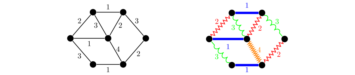
One thing to notice right away is that if a vertex has degree k, then we will need at least k different colors for the edges incident on that vertex. So in general, we have χ' ≥ Δ. A remarkable fact, known as Vizing's theorem, tells us that χ' ≤ Δ+1 for every simple graph, so that there are only ever two possibilities for the edge chromatic number: Δ and Δ +1.

(Vizing's theorem) For any simple graph, χ' is either Δ or Δ+1.

The theorem itself is not too hard to prove. The basic idea involves building up a coloring edge by edge, while adjusting the colors on previously visited edges as we go. But we will skip the details. It is interesting to note that deciding whether χ' is Δ or if it is Δ+1 turns out to be an NP-complete problem.

Note the theorem requires the graph be simple. If the graph has multiple edges, then the theorem may not hold, as in the example below, which has Δ(G) = 8 but χ'(G) = 12.

There is a generalization of Vizing's theorem that works for multigraphs with no loops, namely that χ' can range from Δ through Δ + m, where m is the largest edge multiplicity, the largest number of multiple edges between the same two vertices in the graph.

Edge coloring of common graphs

Just like we did for vertex coloring, it is interesting to examine edge coloring on paths, cycles, complete graphs, and bipartite graphs.

Paths and cycles

Paths and cycles behave the same as for vertex coloring. A few examples are shown below.

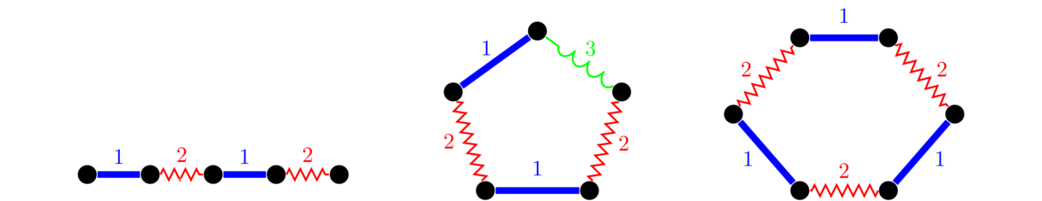
Complete graphs

Complete graphs are more interesting. Shown below are some optimal edge colorings of K₄, K₅, and K₆. Color names have been left out of the figures to avoid cluttering them too much.

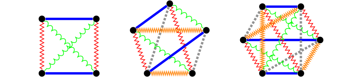
Notice that χ'(K₄) = 3, χ'(K₅) = 5, and χ'(K₆) = 5. Edge coloring complete graphs is much more interesting than vertex coloring them.

For any even n, K_n turns out to have an edge coloring using n-1 colors. Notice in the coloring of K₄ that three colors are used, each color appearing twice. What we do is pair off the vertices repeatedly. The first pairs all four vertices horizontally, the second pairs them vertically, and the third pairs them diagonally. Each pairing corresponds to a different color. These pairings are technically called matchings, which are sets of edges in a graph such that no two share an endpoint. That is, they are independent sets of edges. They are covered in Chapter 7.

It turns out to be possible to do this type of pairing on K_n whenever n is even. We can see this in the example of K₆ above, where the six vertices are broken into three pairs in five different ways, accounting for all 10 edges in the graph, and giving χ'(K₅) = 5.

This pairing off of edges is not possible for odd n. There are an odd number of vertices, so something gets left out. For example, looking at K₅, we see that we cannot use the same color on more than 2 edges. Each time we use a color on an edge, we can't use it on any other edges that share an endpoint with it, so each time we color an edge, we essentially knock out two vertices. Since there are 5 vertices, some vertex will be missed.

Though we'll leave out all the details, the end result is that the edge chromatic number for K₁, K₂, etc. follows the pattern 1, 3, 3, 5, 5, 7, 7, 9, 9, ….

Bipartite graphs

Shown below are edge colorings of some bipartite graphs.

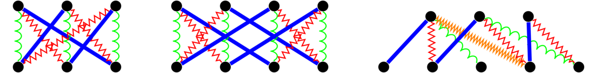
As with complete graphs, for bipartite graphs there is a close relationship between matchings and edge colorings. This is particularly apparent in K_3,3 shown above on the left and on the 3-regular graph in the middle. In each case, we see the vertices in the top partite set matched in three different ways to the vertices of the bottom partite set. For bipartite graphs, there is the following nice theorem.

[König's theorem] For any bipartite graph, χ' = Δ.

Here is the basic idea of the proof: First suppose the graph is regular. By Hall's theorem (see Section 7.4), every regular bipartite graph has a matching that matches each vertex in the one partite set with a unique vertex in the other partite set, so that every vertex is paired off with something else. This is called a perfect matching. We can color each edge in that matching with color 1. Then removing the edges from that matching leaves another regular bipartite graph. We can find another perfect matching, color its edges with color 2, and continue for a total of Δ steps until all edges are used and χ' colors are used in total.

If the graph is not regular, we can add vertices if necessary so that both partite sets have the same size, and then add edges between any vertices in opposite partite sets whose degrees are less than Δ. This creates a regular graph with maximum degree Δ, and then the argument above applies.

Properties of edge colorings

Line graphs

Edge coloring is actually a special case of vertex coloring. In particular, coloring the edges of a graph is equivalent to coloring the vertices of its line graph. In particular, χ'(G) = χ(L(G)). One simple application of this is χ'(C_n) = χ(C_n) since the line graph of a cycle is the cycle itself.

Note that not every graph is the line graph of some other graph. For example, K_1,3 (sometimes called the claw) is not the line graph of any graph (and it is a nice exercise to explain why).

Matchings

We saw matchings appear in our colorings of complete graphs and bipartite graphs. They apply to edge coloring in general.

Recall that for graph coloring we have the result χ ≥ n/α, where n is the number of vertices in the graph and α is the size of the largest independent set. There is an analogous result for edge coloring that uses independent sets of edges (matchings). The size of the largest independent set of edges is denoted α'. Here is the edge coloring analogy of χ ≥ n/α:

For any graph with e edges whose largest independent set of edges is of size α', we have χ' ≥ e/α'.

The proof of this theorem is pretty similar to the proof of the vertex-coloring version. As an example of the theorem in use, it shows that K₅ needs at least 5 colors. In that graph, we have α' = 2 and e = 10, so χ' ≥ 10/2 = 5. For K_n in general, we have α' = floor(n/2) and e = n(n-1)/2, so we get χ'(K_n) ≥ n.

Applications

Just like with vertex coloring, there are applications of edge coloring, especially to scheduling problems. Here is one example. Suppose six teams play in a round-robin tournament, where each team plays each other team once. We want to schedule matches so that no team plays two matches in a day.

The solution is to create a graph where the teams are vertices, an edge represents a match between two teams, and an edge's color is the day that the match should occur. If two edges that share an endpoint were to get the same color, then that would correspond to a team playing two games on the same day.

The graph generated is K₆, which can be colored with 6 colors, with the specific coloring giving us the exact schedule of matches.

Further details on coloring

The name “coloring” might seem to be an unusual one. It comes from one of the earliest and most influential problems in graph theory, called the four color problem. The problem originated in 1852 when a certain Francis Guthrie noticed while coloring maps of the counties of England that he only needed four colors to color them so that bordering counties got different colors. He wondered if this was true for all maps. This set in motion a century-long search for a solution, which ended in 1976 with a computer-aided proof by Kenneth Appel and Wolfgang Haken. The whole story is an interesting one, about which books have been written. Attempts to prove the theorem led to the development of many parts of modern graph theory.

The relation to graph theory is that maps can be represented by graphs by making each region (county, state, etc.) a vertex and adding an edge between vertices whenever their corresponding regions border each other, as in the example below.

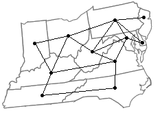
Coloring the regions is then the same as “coloring” the vertices of the graph. Graphs obtained from maps in this way are planar graphs, which are the subject of the next chapter.

Planar Graphs

Definitions and properties

This chapter is about trying to draw graphs so that none of their edges cross. For example, the usual way to draw K₄ has two edges crossing, as in the figure below on the left. However, we can move some of those edges around to remove the crossings, as shown in the middle and right below.

Here is another example, showing two ways to draw the cube graph without crossings. One thing we can do is visualize sliding and shrinking one of the cube's squares so it fits inside the other. Alternately, notice that the cube has a Hamiltonian cycle. We start by drawing the cycle, with the vertices arranged around a cycle and then try to get the last few edges to work out.

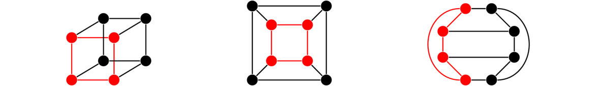
There is a fun game called Planarity, available online and as an app, that is all about dragging around vertices to get rid of all the crossings.

It is not possible to draw all graphs without crossings. For example, K₈, shown below, has 56 edges and only 8 vertices. It doesn't seem like there could be any way to avoid all the crossings.

So we have the following definitions.

A plane graph is a graph drawn so that no edges cross. A graph is called planar if it is possible to draw the graph as a plane graph.

This definition is somewhat vague since we haven't really said what it means to “draw the graph” or what “crossing” means. Instead, we will hope the reader has an intuitive idea of what these things mean. See the Wikipedia page on graph embedding for the precise mathematical details, which can get a little hairy.

The term “planar” comes from the fact that we are drawing (or embedding) the graph in the plane, like on a piece of paper. At the end of the chapter we will consider drawing graphs on other surfaces, like toruses.

Euler's formula

A plane graph divides the plane into two-dimensional regions, called faces. Shown below is a graph and five faces, A, B, C, D, E along with a sixth special face, O, called the outside face.

Euler was interested in the Platonic solids, shown below.

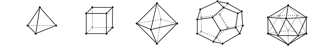
The five Platonic solids are the tetrahedron, cube, octahedron, dodecahedron, and icosahedron, with 4, 6, 8, 12, and 20 faces respectively.

The Platonic solids are regular polyhedra. They are the three-dimensional analogs of regular polygons, where every face is an identical polygon. For instance, in a cube, all six faces are squares. In the dodecahedron, all 12 faces are identical pentagons. A famous result, that we will actually prove in shortly, is that the five Platonic solids are the only regular polyhedra. This may be a bit surprising as there are infinitely many regular polygons, but only five regular polyhedra.

Euler noticed that if you add the number of vertices and faces and subtract the number of edges (v-e+f) for these solids, the result always comes out to be 2. The graph theoretic analog of this is shown below, where the five Platonic solids are embedded in the plane as graphs. Notice that v-e+f for each of these graphs comes out to 2.

This fact is not just true about Platonic solids—it is true about any plane graph. You can check this by looking at any of the plane graphs drawn earlier in this chapter or elsewhere. This result is called Euler's formula.

We can see why this might be true: First, It works for any tree since a tree on v vertices has v-1 edges (as we saw in Section 3.2) and 1 face, and so v-e+f = 2. Next, imagine adding edges to the tree. Any time we add an edge between two vertices of a plane graph, we create exactly one new face, so e and f increase by 1, while v doesn't change, leaving v-e+f fixed at 2. Notice in the figure below how adding the dashed edge creates a new face, F.

Further, if we add a leaf to a plane graph, this increases e and v by 1, but keeps f and also v-e+f fixed. This argument, while intuitively clear, is a little tricky to make rigorous because we would have to prove that every graph can be built up in this way by starting with a tree and adding edges and leaves. Instead, in our induction proof below we work in the other direction, thinking about removing things from a plane graph instead of adding things.

Here is the statement of the Euler's formula and a proof.

(Euler's formula) For any connected plane graph, the numbers of vertices v, edges e, and faces f satisfy v-e+f = 2.

The proof is by induction on the number of faces f. For the base case f = 1, a graph with only 1 face must have no cycles, and hence is a tree. In a tree, we have e = v-1, and so v-e+f = 2.

Now assume the formula holds for any connected plane graph with f-1 faces, and consider a connected plane graph with f faces. Let v and e be the number of vertices and edges of this graph. This graph must contain a cycle, as otherwise the graph would be a tree and there would be only 1 face. Remove any edge of that cycle. Doing so merges two faces (possibly a face with the outside face). This has the effect of reducing the number of edges and faces by 1, while leaving the number of vertices fixed. Since the number of faces is now f-1, the induction hypothesis applies and we have v-(e-1)+(f-1) = 2. Simplifying gives v-e+f = 2.

Another nice proof of Euler's formula runs by induction on the number of vertices and involves contracting an edge, which has the effect of reducing the vertex and edge counts by 1, while leaving the face count fixed, thus having no net effect on the count v-e+f.

Notice that there are some technical details that we are brushing aside. For instance, in the face-induction proof, we said that a tree has only one face, and we also said that removing an edge from a cycle merges two faces. While these statements may be intuitively obvious, they take quite a bit of work to prove, usually relying on something called the Jordan curve theorem.

Note that Euler's formula doesn't hold for disconnected graphs, but a variant of it does, namely v+e-f = c+1, where c is the number of components. We can get this easily from Euler's formula by adding c-1 edges to the graph in order to connect up all the components. This will not affect the number of vertices or faces, so in this new connected graph Euler's formula gives us v+(e+c-1)-f = 2, which simplifies to v+e-f = c+1.

Consequences of Euler's formula

Platonic solids

Euler's formula can be used to show that the five Platonic solids are the only regular polyhedra. To show this, first note that in a regular polyhedron the degree of each vertex and number of edges around each face must be the same throughout the entire figure. Let j be the degree of each vertex and k be the number of edges around each face. We have k ≥ 3 since the faces of a polyhedron are polygons, which must have at least 3 sides. This also implies j ≥ 3.

Each of the v vertices has degree j, so by the degree sum formula, we have jv = 2e. Further, each edge lies on the boundary of exactly two faces, so kf = 2e. Plugging these into Euler's formula and simplifying gives e(2/k - 1 + 2/j) = 2. Since e and 2 are positive, the term in parentheses must also be positive, which after a little algebra means 2(j+k) > jk.

This inequality is fairly limiting since the right side grows much more quickly than the left. For instance, if j = k = 5, the inequality says 20 > 25, which is false. It is not too much work to check that only the following possibilities work for j and k in this inequality: (3,3), (3,4), (4,3), (3,5), (5,3). These correspond to the tetrahedron, cube, octahedron, dodecahedron, and icosahedron, respectively.

Inequalities for planar graphs

We can use Euler's formula to get the following inequalities that we can use to show certain graphs are not planar.

Any simple plane graph with v ≥ 3 vertices and e edges satisfies e ≤ 3v-6.

First, suppose the graph is connected. Since the graph is simple, connected, and has at least 3 vertices, every face must have at least 3 edges around its boundary. Thus the sum of all the face lengths (number of edges around the face's boundary) in the graph is at least 3f. Moreover, each edge in the graph can be on the boundary of at most 2 faces (1 if it's a cut edge, 2 otherwise), so when we sum the face lengths, each edge gets counted at most twice. Putting these two facts together, we get 2e ≥ 3f. If the graph is connected, we can plug this into Euler's formula to get 2 = v-e+f ≤ v-e+²/₃e and simplify to get e ≤ 3v-6.

If the graph is not connected, we can add some number of edges to it to make it connected. By the paragraph above, this new connected graph must have no more than 3v-6 edges and so the original (which has less edges) must also have no more than 3v-6 edges.

Any triangle-free simple plane graph with v ≥ 3 vertices and e edges satisfies e ≤ 2v-4.

The proof of this theorem is the same as for the previous theorem except that if there are no triangles, then every face has at least 4 edges around its boundary. So 2e ≥ 4f, and the algebra works out to give us e ≤ 2n-4. In particular, bipartite graphs are triangle-free, so we can use this rule instead of the other for bipartite graphs as it is stronger.

These theorems say that for a given number of vertices, once the number of edges gets too high, the graph has no chance of being planar. There are just too many edges and not enough vertices to draw the edges without crossings. Further, these are necessary, but not sufficient conditions for a graph to be planar. That is, we can only use these theorems to show that a graph is not planar.

Let's apply the first inequality to K₅. Here we have v = 5 and e = 10, and the inequality e ≤ 3v-6 becomes 10 ≤ 9, which just barely does not hold. This means that K₅ is not planar. If you try drawing K₅ as a planar graph, you'll notice that you have one edge left over that you can't draw without crossing.

Now we'll look at the complete bipartite graph K_3,3. The inequality e ≤ 3v-6 holds for this graph, so it doesn't help us at all. But let's apply the second inequality e ≤ 2v-4. Here we have v = 6 and e = 9, and the inequality e ≤ 2v-4 becomes 9 ≤ 8, which does not hold. Thus K_3,3 is not planar.

This answers a famous old puzzle called the “three utilities problem.” In that problem, there are three houses and three utilities: water, gas, and electric. We want to connect each house to each utility without having any utility line cross another. Is it possible? A partial attempt at a solution is shown below.

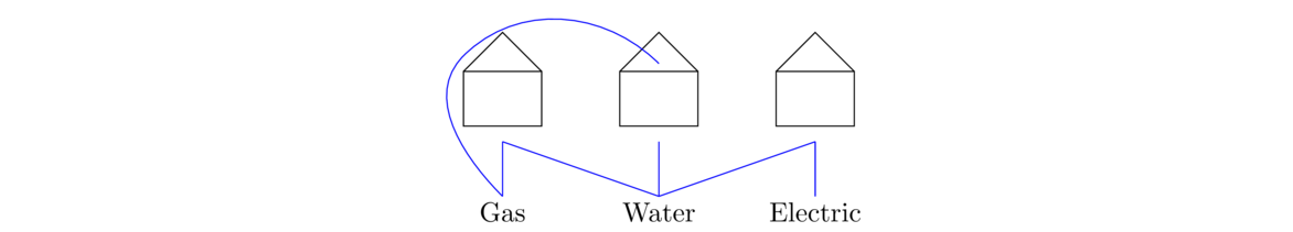
Modeled as a graph, this problem is asking if K_3,3 is planar, which we now know to be false, so the puzzle has no solution.

A limit to vertex degrees

We can use Euler's formula to get the following useful fact.

Every simple planar graph has a vertex of degree 5 or less.

Suppose, on the contrary, that every vertex has degree 6 or more. By the Degree sum formula, the sum of the vertex degrees is twice the number of edges. Since the sum of the vertex degrees is at least 6v, we have 2e ≥ 6v, and hence e ≥ 3v. But this contradicts that e ≤ 3v-6 for a planar graph.

People often confuse what this theorem says. It says that in every planar graph, there is at least one vertex that has degree 0, 1, 2, 3, 4, or 5. The other vertices in the graph might have very high degree or low degree or whatever. It might be a little surprising to think that every planar graph has to have a vertex of relatively low degree, but the alternative (every vertex with degree 6 or more) forces too many edges in the graph and hence too many crossings.

Kuratowski's theorem

The graphs K₅ and K_3,3 turn out to be extremely important in terms of telling which graphs are planar. Clearly if one of these is a subgraph of a graph, then that graph can't be planar. But there are other possible ways they can show up, like below.

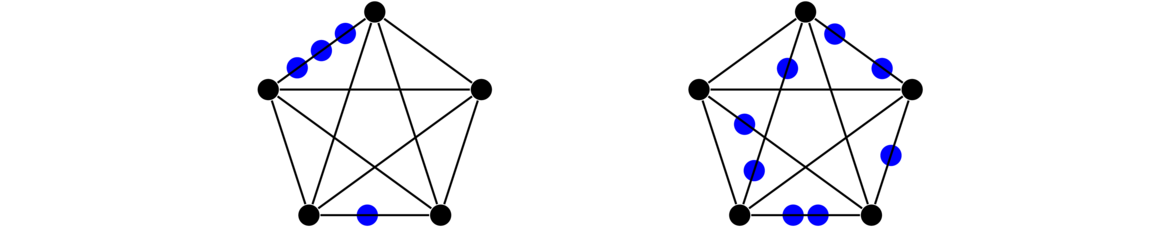
What we've done is essentially added vertices into the edges of K₅. We haven't done anything that would help us get rid of the crossings of K₅, so these graphs are also not planar. This process of adding vertices into edges is called subdivision. Here is the formal definition.

A subdivision of an edge uv is the process of creating new vertices w₁, w₂, … w_n and replacing edge uv with edges uw₁, w₁w₂, … w_n-1w_n, and wv. A subdivision of a graph is a new graph obtained by subdividing some of the edges of the graph.

The interesting part of the story here is that K₅, K_3,3 and their subdivisions are the only obstacles to a graph being planar. This is known as Kuratowski's theorem. It is stated below without proof, as the proof is fairly involved.

(Kuratowski's theorem) A graph is planar if and only if it does not contain a subgraph isomorphic to K₅, K_3,3 or a subdivision of either.

Therefore, to show a graph is not planar, it suffices to find K₅, K_3,3, or a subdivision of one of them in the graph. However, this can take some work. Here is an example.

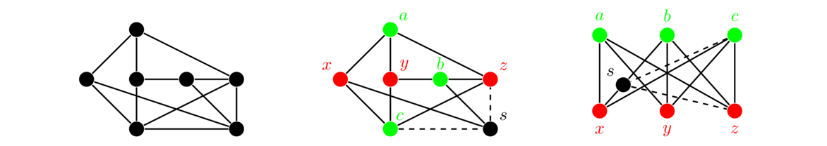
On the left is the graph we are trying to show is nonplanar. In the middle, we have found a K_3,3 subdivision. One partite set is {a,b,c} and the other is {x,y,z}. We have all the edges of K_3,3 present in the graph except for edge bx. However, we have a path from b to s to x, so that is our subdivided edge. The subdivision is redrawn on the right to look more like the way K_3,3 is usually drawn. Note that edges sc and sz are not needed for the subdivision, so we have drawn them with dashed lines.

Here is another example:

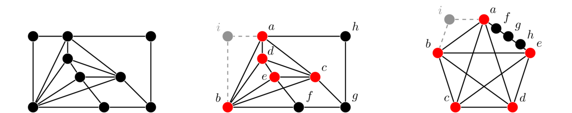
Here the graph contains a K₅ subdivision, which makes it nonplanar. The vertices a, b, c, d, and e form K₅ and vertices f, g, and h subdivide the edge from a to c. Vertex i is not used in the subdivision.

Here is the Petersen graph as an example:

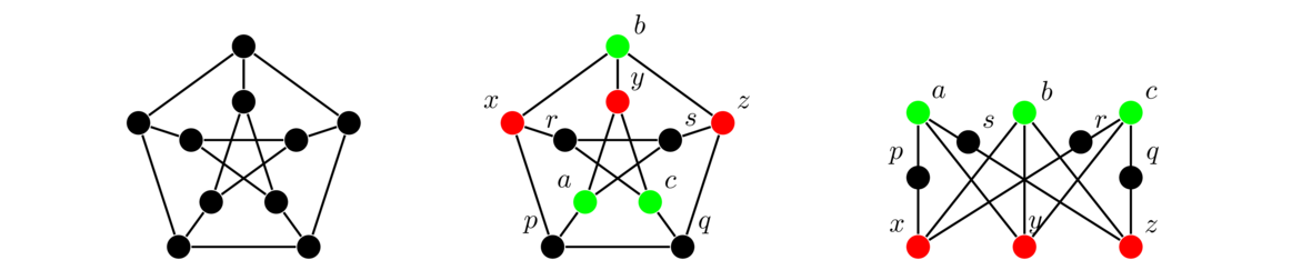
We see that the Petersen graph is a subdivision of K_3,3. The vertices a, b, and c form one partite set, and the vertices x, y, and z the other. The rest of the vertices go towards subdividing edges. This shows the Petersen graph is nonplanar.

Note: A common mistake is to try to use the same vertex to subdivide multiple edges. That is not allowed. A vertex can only be used towards subdividing one edge.

More on planarity

Wagner's theorem

There is an interesting variation of Kuratowski's theorem, called Wagner's theorem, that uses graph minors instead of subdivisions. A graph minor is a graph you obtain from another by deleting vertices and contracting edges.

(Wagner's theorem) A graph is planar if and only if it does not contain a K₅, K_3,3, or a minor of either.

The Petersen graph, shown below, has a K_3,3 minor. We contract the highlighted edges xp, cr, as, and qz to obtain the graph on the right, which is K_3,3.

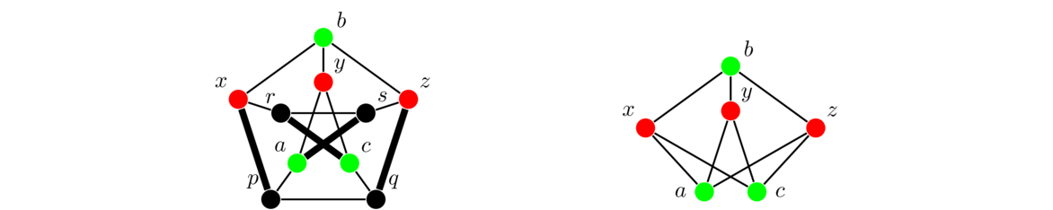
It also has a K₅ minor, which can be seen by contracting each of the edges that lead from the outside cycle to the inside cycle.

Fáry's theorem

There is a surprising result called Fáry's theorem that says that curved lines are never needed to draw a planar graph. Every planar graph can be drawn using only straight lines.

The proof relies on induction. At the induction step we assume that any planar graph on n vertices can be drawn with only straight lines and look at an (n+1)-vertex planar graph. We locate and remove a vertex v whose degree is at most 5, which we know exists in a planar graph by Theorem 29. By the induction hypothesis, we can draw the remaining graph with only straight lines, and now we just have to fit v back in. Since its degree is at most 5, if we look at its neighbors, we can treat them as the vertices of a polygon with at most 5 sides. We have to show that we can find a place inside that polygon in which to fit v so that it can “see” all the other vertices. This can be done by looking at the various possible shapes of triangles, quadrilaterals, and pentagons, which break down into just a few general cases.

Crossing number

Graph theorists also study the crossing number of a graph, which is the minimum number of crossings needed to draw the graph in the plane. For example, the crossing numbers of K₅ and K_3,3 are 1, as shown below.

Determining crossing numbers is actually quite difficult, with a lot of open problems. For instance, the crossing number of K_m,n is not known in general. It is suspected that the value is floor(ⁿ/₂)floor(^n-1/₂)floor(^m/₂)floor(^m-1/₂), but no one has been able to prove it. The problem is called the Turán brick factory problem, as the mathematician Pál Turán thought of it while working in a brick factory. There he had to push bricks around in a wagon, and crossing over wagon ruts in the ground was difficult. The crossing number of the complete graph K_n is also not known in general.

Applications of planarity

As we saw above in the brick factory problem, crossings are often not desirable in real-life applications. Planarity thus has applications in a variety of places. For instance, graphs are often used to visualize data, and they are easier for people to follow when there are few crossing edges. Planarity can also be useful in the design of transportation networks, where we don't want unnecessary intersections. Further, crossings of electric wires, especially in chips is often a bad thing, leading to interference, so planarity applies here as well.

Algorithms

Graph theorists are interested in fast algorithms to determine if a graph is planar as well as algorithms to draw planar graphs without crossings. The simple approach of looking for K₅ or K_3,3 subdivisions is unfortunately very slow, potentially taking an exponential number of steps. Searching for minors can be even worse. However, various approaches were developed starting in the 1960s that run much more quickly, in polynomial time. We won't get into the details here.

The four color theorem

One of the most famous problems in graph theory is the four color theorem. As mentioned in Section 5.5, the idea is to try to color maps so that adjacent regions (countries, states, etc.) get different colors. Also as mentioned in that section, we can covert the map to a graph by turning the regions into vertices with an edge between vertices indicating that the regions they represent share a border. We assume that a region is contiguous (i.e. not in two disconnected parts like the contiguous U.S. and Alaska). This means the resulting graph is planar. The four color theorem states that every planar graph can be colored in four colors or less.

Note that some planar graphs, like K₄, need four colors, while others can be colored with fewer. While proving the four color theorem is well beyond our means, we can come close, proving that we can color every planar graph with 5 colors or less.

The six color theorem

We'll start, though, by proving that we can color any planar graph with 6 colors or less. We use induction on the number of vertices. The base cases are planar graphs with 6 vertices or less, which can certainly be colored with 6 colors or less. Now assume that we can color all planar graphs on n vertices with 6 colors or less and consider an (n+1)-vertex graph. Since it is planar, by Theorem 29 it has a vertex v of degree 5 or less. Remove that vertex, leaving an n-vertex planar graph. Then by the induction hypothesis, we can color it with 6 colors or less. We can use this coloring on our full graph if we can find a way to color v. And since v has no more than 5 neighbors, one of the 6 colors has not been used on one of its neighbors, so we have a color available for it. And that's the six color theorem.

The five color theorem

If we work a little harder with the same approach, we can prove the five color theorem. The proof is still by induction in the exact same way, but at the inductive step, the vertex v might have 5 neighbors, all of which get different colors, and there is no obvious choice then for a color to use on v.

If we can find a way to recolor the graph so there are only 4 colors on the neighbors of v, then we can color v. To this end, we can assume that the colors on the neighbors v₁, v₂, v₃, v₄, and v₅ of v are named 1, 2, 3, 4, and 5, in clockwise order around v.

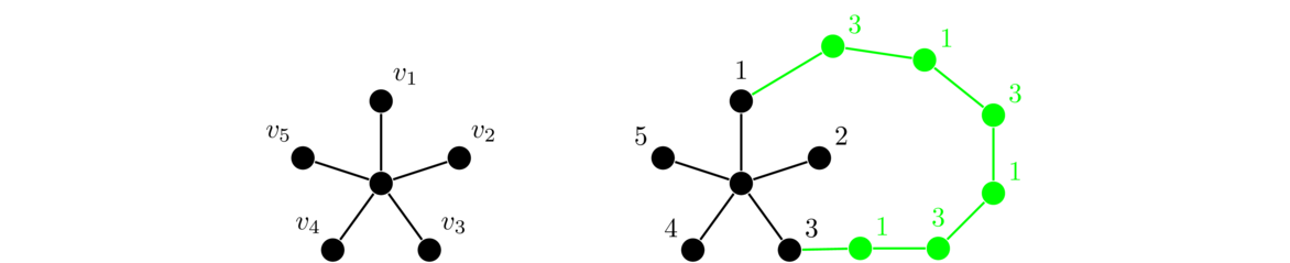
Perhaps we can recolor the graph so that v₁ and v₃ are both colored with a 1. We can try by this looking at the component of G-v containing v₁ and swapping colors so that any vertex in that component that is currently colored with a 1 gets colored with a 3 and all the vertices colored with a 3 get colored with a 1. This will work to eliminate color 1 from the neighborhood of v unless it turns out that v₃ is also in that component and there is some path from v₁ to v₃ in which the colors alternate 1, 3, 1, 3, etc. This is shown above.

If such a path exists, then we move on to v₂ and v₄ and try the same approach, this time trying to swap colors 2 and 4. We will be able to color v₄ with a 2 unless there is a path from v₂ to v₄ in which the colors alternate 2, 4, 2, 4, etc. However, now we have a problem. This path along with v forms a cycle in the graph as does the alternating 1, 3 path. But take a look at the graph above on the right. It is not possible to have both of these cycles in the graph without them crossing over each other, either at a vertex or at an edge. But they can't cross at a vertex as the one path is colored solely with 1 and 3 and the other is colored solely with 2 and 4. They can't cross at an edge because the graph is planar. Therefore, we can't have both the 1, 3 path and the 2, 4 path in the graph. So we must be able to remove a color from the neighborhood of v and hence we can color v, leading to a 5-coloring of the graph.

The four color theorem

Notice how in the proof color #5 does not make too much of an appearance. This gives us hope that this approach might work to prove the four color theorem. That is exactly the approach used by Alfred Kempe in 1879. He is the one who came up with the idea of using those alternating paths, which are now called Kempe chains. Kempe's 1879 proof was widely celebrated and helped get him elected to the Royal Society. However, in 1890, Percy Heawood found a flaw in Kempe's proof. Kempe had used some intricate manipulations of his eponymous chains and one of the cases involved chains that could interleave. Kempe had missed that possibility (as did everyone who checked his proof and many people who later tried to prove the four color theorem). His proof was therefore incomplete and was not able to be repaired. Heawood did use it to give a proof of the five color theorem that is essentially the same as the one presented above.

Kempe's ideas, however, formed the basis of the proof that eventually worked, though it took the better part of a century for the details to be worked out. Here is the basic idea: First we only need to focus on maximal planar graphs, graphs where we have added as many edges as possible to the point that we can't add any more without forcing the graph to be nonplanar. We then seek a minimum counterexample, the smallest planar graph that can't be colored with 4 colors or less, and try to show that no such counterexample can exist. To do this, we look for what's called an unavoidable set, a set of graphs such that every maximal planar graph with at least five vertices must contain at least one graph in that set. And we then try to show that every graph in that set is reducible, that is that it cannot be contained in a minimum counterexample.

With this terminology, Kempe's approach was essentially that he found an unavoidable set that consists of C₃∨ K₁, C₄∨ K₁, and C₅∨ K₁, and his proof attempted to show that they were all reducible, though it failed with C₅∨ K₁. Further attempts at finding unavoidable sets throughout the 20th century resulted in some progress, like showing the four color theorem holds for planar graphs with at most 36 vertices. It wasn't until the 1970s that Kenneth Appel and Wolfgang Haken, based on ideas of Heinrich Heesch, put together a computer search for unavoidable sets. Previous attempts weren't amenable to such an approach, but Appel and Haken managed to find an approach that could work given the computing power of that era.

Their program, which required over a thousand of hours of supercomputer time, succeeded in finding an unavoidable set of size 1936, all of which they verified to be reducible. Later work by Robertson, Sanders, Seymour, and Thomas brought this down to an unavoidable set of size 633, small enough to be checked in under a few hours on a modern laptop.

The announcement of Appel and Haken's proof produced an outcry from some mathematicians, this being the first major theorem to be proved with significant computer assistance. They complained that the proof was too large to be verified by hand and that it might be subject to computer error. Nowadays, few mathematicians doubt the correctness of the proof, though many mathematicians would prefer a simpler, more aesthetically pleasing proof.

Embedding graphs on surfaces

The term “planar” comes from the fact that we are trying to draw graphs in the plane. It is interesting to try drawing graphs on other objects. First, we can ask about drawing graphs in 3D. This turns out to have the simple answer that any graph can be drawn in 3-space without crossing edges. There is just so much room that we can always avoid crossings.

The next object we might try is the sphere. This turns out also to have a simple answer, namely that a graph is planar if and only if it can be drawn on a sphere. Topologically speaking, the plane behaves the same as a sphere with a point cut out of it. It is possible to poke a point out of the north pole of a sphere and unroll it into the plane. This is the same principle by which it is possible to draw a map of the earth on a piece of paper.

The first common object that we come to with an interesting answer is the torus, a doughnut shape, shown below.

Visualizing graphs on a torus can sometimes be a pain. Instead, we use a convenient representation of the torus on a piece of paper. Starting with a piece of paper, we can construct a torus by first folding around two sides of the paper to create a cylinder and then folding the cylinder around in the same way to connect the two ends together. This is shown in the figure below.

The left and right parts of the paper are pasted (or identified) together in creating the torus, and to indicate that we use single arrows, like shown in the figure below. We use double arrows to represent that the top and bottom parts are pasted together. So we can think of a torus like a piece of paper where the right side wraps around to the left and the bottom wraps around to the top. This is a little like some video games, like Pacman.

We can embed many graphs on a torus that we cannot embed in the plane. An example is shown below.

Notice how two of the crossings are replaced by wrapping around the top of the rectangle and the other is replaced by going around the side. Here are two more examples, embeddings of K₅ and of K_3,3.

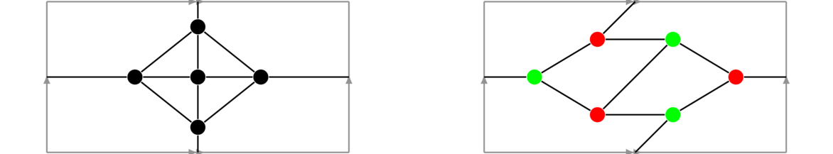
We can go further, being able to embed K₆ and K₇, with some cleverness. However, this is as far as we can go on a torus, as K₈ cannot be embedded on it.

The torus behaves topologically the same as a sphere with a handle. That is, if we imagine a torus made of clay, it is possible to deform that torus by stretching and reshaping the clay until we have a sphere with a handle. It is never necessary to cut or break off any of the clay. This is the source of the classic joke about a topologist not being able to tell the difference between a coffee cup and a doughnut. Shown below is K₅ embedded on the torus and on a sphere with a handle.

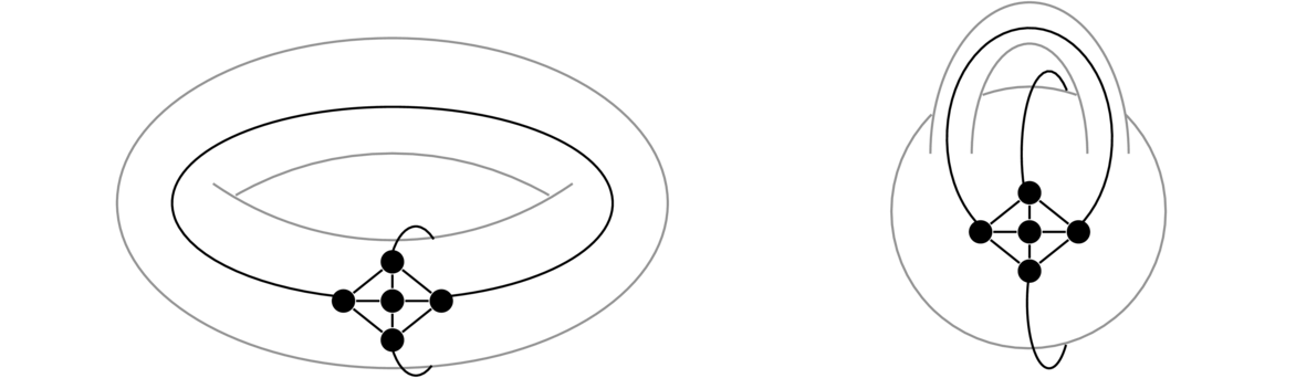
From here, we see why the torus allows us to embed things that we can't embed in the plane: the handle allows us to add extra crossings. This, of course, leads to a natural generalization: more handles. A sphere with two handles is equivalent to a double torus.

With this extra handle, we can now embed K₈. In fact, given any graph, we can take a sphere and keep adding handles until we have enough to avoid all crossings. The minimum number of handles needed is called the genus of the graph. For K_n, the genus turns out to be ceiling(^(n-3)(n-4)/₁₂) and for K_m,n, it is ceiling( ^m-2)(n-2)/₄). In particular, on a torus we can embed K_3,3 and K_4,4 but not K_5,5.

Finally, we note the interesting Heawood map coloring theorem. It was formulated by Heawood when he pointed out the flaw in Kempe's proof, but it wasn't fully proved until the 1960s and 1970s. It generalizes the four color theorem by stating that any graph that can embedded be a sphere with g handles (also known as a surface of genus g) can be colored with at most floor((7 + √1+48g) / 2) colors. The genus g = 0 case is the four color theorem. The genus g = 1 case is the torus and the formula works out to 7. So any graph that can be embedded on a torus can be colored with 7 colors or less. This bound is sharp in that there are graphs (like K₇) that require 7 colors. For the double torus the value works out to 8. The branch of math that deals with all of this is called topological graph theory.

Matchings and Covers

Definitions and properties

We have seen independent sets before. Here is their definition again.

An independent set in a graph is a subset of its vertices in which no two vertices are adjacent. An independent set of edges, usually called a matching, is a subset of its edges in which no two edges share an endpoint.

An example independent set is shown below on the left. The highlighted vertices, d and f, form an independent set. On the right, the highlighted edges, af, bc, and ed, form an independent set of edges.

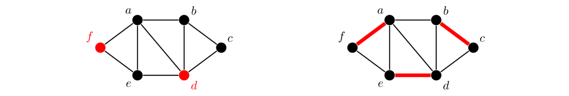
For example, suppose we have a graph whose vertices represent people, with edges between vertices indicating that the corresponding people know each other. An independent set in this graph represents a collection of people that are all strangers to each other. A matching in this graph pairs off some or all of the people with someone else they know, with no one appearing in multiple pairs. Often we are looking for a perfect matching, where everyone is matched to someone, but that isn't always possible.

Closely related to independent sets are covers, defined below.

A vertex cover of a graph is a subset of vertices such that every edge in the graph has an endpoint in that subset. An edge cover is a subset of edges such that every vertex in the graph is an endpoint of some edge in the subset.

An example is shown below. In the figure on the left, the highlighted vertices a, c, d, and e form a vertex cover. Every edge in the graph is incident on one of those vertices. In the graph on the right, the highlighted edges ef, ad, and bc form an edge cover.

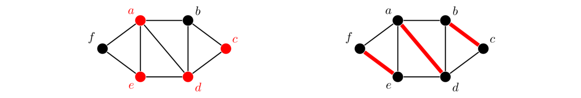
A nice analogy for vertex covers is the following: think of the edges as hallways and we want to place guards at vertices so that every hallway (edge) is guarded. In an edge cover, we place guards in the middle of the hallways so that each intersection (vertex) can be seen by someone.

Note the following notation:

α	size of largest independent set
α'	size of largest independent set of edges (matching)
β	size of largest vertex cover
β'	size of largest edge cover

Stars (K_1,m), are extreme cases for all four parameters. Shown below is the star K_1,5.

In a star with m leaves, we have α = m, since we can take all of the outside vertices as an independent set. This is as large a proportion of a graph's vertices as is possible to be contained in an independent set, if the graph is connected. We have α' = 1 in any star, since every edge has the center as an endpoint, and that center can only be used once. This is as small as α can possibly be in a graph that contains any edges. We have β = 1 as the center vertex covers all edges, and we have β' = m, since we need to use every edge in the graph in order to cover all the outside vertices.

Here are a couple of simple facts about matchings and edge coverings.

For any graph, we have α' ≤ n/2 and β' ≥ n/2.

The first part is true because each edge of a matching knocks out two vertices (its endpoints) and once a vertex is used in a matching, it can't be used again. The second part is true because any edge can cover at most two vertices (its endpoints).

Independent sets and coverings turn out to be closely related to each other. Here are two relationships:

[Gallai identities] For any graph with n vertices we have

α+β = n
α'+β' = n, provided the graph has no isolated vertices.

Let's look at #1 first. Suppose S is an independent set. Then its complement, S = G-S, is a vertex cover. This is because there are no edges between vertices in S, so every edge of the graph must be between vertices of S, making S a vertex cover. This works the other way as well—the complement of a vertex cover is an independent set. Thus, if we take a maximum independent set S, then its complement is a minimum vertex cover since the complement of any smaller vertex cover would give a larger independent set than S. Since |S|+|S| = n, we get α+β = n.

For example, in the graph below, {d, f} is an independent set, while its complement {a, b, c, e} is a vertex cover.

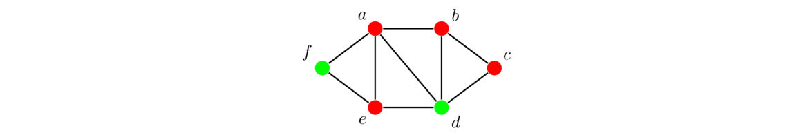
For #2, first note that it is impossible to edge cover an isolated vertex, so we need to assume there are no isolated vertices. To prove α'+β' = n, start with a matching of size α'. We can build on it to create an edge cover. That edge cover consists of every edge of the matching along with one additional edge for each vertex not in the matching, taking whichever edge incident on that vertex that we want. This cover consists of the α' edges from the matching along with at most n-2α' additional edges (this is because each edge of the matching covers two vertices, so there are n-2α' vertices left uncovered). This is an edge covering of size α'+(n-2α'), and it is at least as large as the minimum edge covering, so we have

β' ≤ α'+(n-2α'), which simplifies to α'+β' ≤ n.

See the figure below for an example of this. On the left is a matching and on the right is the matching along with the added edges to create an edge cover.

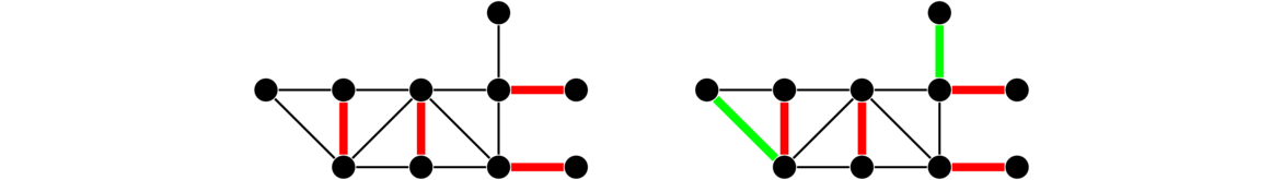
We now need to show α'+β' ≥ n, which would then prove #2. To do so, start with an edge cover of size β'. Since this edge cover is of minimum size, it cannot contain a path of length 3 because the middle edge of such a path would be redundant. So the subgraph formed by the edge cover can contain only paths of length 2, meaning it consists purely of stars. We create a matching from this cover by taking one edge from each star. Assume there are k stars. Each edge of the cover goes from a central vertex of a star to a leaf of that star. There are β' such edges, which counts all the non-central vertices, and k counts all the central vertices. This gives β'+k = n. Since k is the size of the matching we created, we have α' ≥ k and hence β' + α' ≥ n, as desired.

The figure below gives an example of this. The edge covering, highlighted on the left with zigzagged edges, consists of three stars with centers a, b, and c. The matching we derive from this is highlighted on the right.

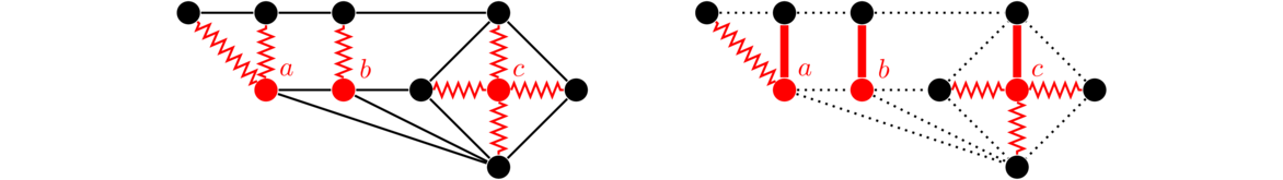
Bipartite matching and the Augmenting Path Algorithm

Matchings in bipartite graphs have a lot of applications. For instance, suppose we have a group of people and a group of jobs, where we want to assign each person a single job. We can represent this as a bipartite graph with one partite set being people and the other being jobs. An edge between a person and job indicates that person can do that job. We want a matching that matches as many people to jobs as possible.

Here is another example: Suppose we have several people that want to give presentations and we have a limited number of time slots available. Each person is only available for certain time slots, and we want to allow as many people to give their presentations. As a graph, the people are one partite set, the time slots are another, and an edge between a person and a time slot indicates they are available at that time slot. A matching would assign time slots to people.

In this section we will work out the details of an algorithm, called the Augmenting path algorithm that finds maximum matchings.

Relation between matchings and covers

One of the keys to finding maximum matchings is the relationship between matchings and vertex covers given below.

In any graph, α' ≤ β.

In a vertex cover, no vertex can cover more than one edge of a matching, since if a vertex did so, then there would be two edges of a matching incident on the same vertex, which is impossible. So we will need at least as many vertices in our cover as edges in any matching.

In particular, every vertex cover is at least as large in size as every matching. So if we have a matching and we find a vertex cover with the same size as that matching, then we know that the matching must be maximum (and that the vertex cover must be minimum).

Augmenting paths

In everything that follows, assume the two partite sets are X and Y. In the figures, X will be the top partite set and Y will be the bottom. Below is a bipartite graph with two matchings highlighted.

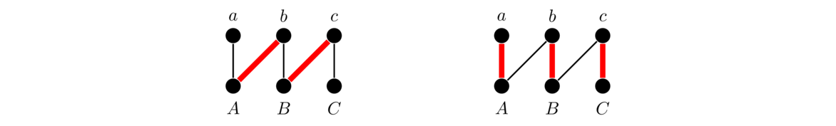
We can use the matching on the left to generate the matching on the right. The trick is to try to find a path, called an augmenting path, that starts at an unmatched vertex of X, ends at an unmatched vertex of Y, and alternates between edges not in the matching and edges in the matching. In the graph above, that path is aAbBcC. If we flip-flop the edges on the path so that matched edges become unmatched and unmatched edges become matched, we will create another matching that is one edge larger. This is the matching shown on the right.

Below is another example. On the left is a matching, and on the right is a better matching. The path eDdBbE is an augmenting path in the left graph. Along that path dD and bB are in the matching, while eD, dB, and bE are not in the matching. Reverse this to get the matching shown on the right.

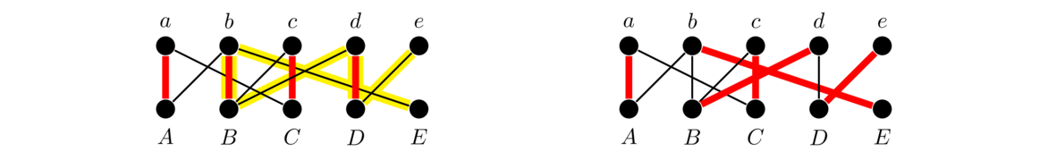
So augmenting paths can be used to make a matching larger. A natural question arises: if we start with a matching that is not the largest possible, is there an augmenting path in the graph? The answer is yes. The proof of this will come later. So we have an approach to finding the largest matching in a graph: start with an empty matching, and increase it one edge at a time by searching for augmenting paths until there are no augmenting paths to be found.

We can do this search by starting at an unmatched vertex of X, following an edge not in the matching, then an edge that is in the matching, then one not in the matching, etc. until we hopefully get to an unmatched vertex of Y. If we get stuck, then we try a different route from that unmatched vertex of X or try a different unmatched vertex of X. We can do this search systematically to make sure that we have explored all routes.

Let's use it to find a maximum matching in the graph below.

Suppose we start with vertex a. We follow an edge down to vertex A , find A to be unmatched and add edge aA to the matching. This is a very simple augmenting path. We then search from vertex b, find B unmatched, and add bB to the matching. The result of these two steps is shown in the leftmost graph below.

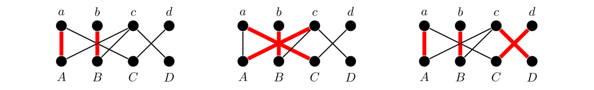
Next we search from vertex c. If we go from c to B to b, we get stuck without finding an augmenting path. So we go back and try the path cAaC. This path is augmenting, so we swap edges to get the matching shown in the middle. Finally, searching from vertex d, we find the augmenting path dCaAcD and swapping edges gives the matching on the right, which includes every vertex.

Making sure the matching is maximum

It would be nice to be sure that the algorithm always works. Recall that if we can find a vertex cover the same size as a matching, then that means the matching is maximum. To do this, we will keep track of the vertices as the algorithm reaches them. Specifically, we keep track of two sets, S and T. The set S is initialized with all the unmatched vertices of X, and T is initially empty. Then every time during our search we visit a vertex, we add it to S if the vertex is in X and add it to T otherwise. If our algorithm finds no augmenting path, then (X-S) ∪ T is a vertex cover with the same size as our matching.

An example is shown below.

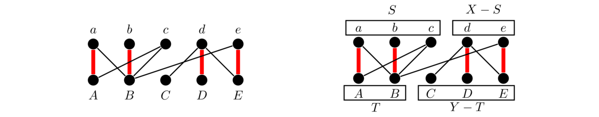
The matching shown is maximum. In our search for an augmenting path, we would start with S = {c} and T empty. We could try the path from c to B to b. That's a dead-end, but as we visit b and B, we add them to T and S, respectively. Then we try the other edge from c, following the path cAaBb. Here we add a to S and A to T, leaving us with S = {a,b,c} and T = {A,B}.

Then (X-S) ∪ T is a vertex cover of size 4. This can be easily checked. Notice that (X-S) and T must cover all edges except those from S to Y-T. However, there are no edges between those two sets. Notice also that each vertex of X-S and of T corresponds to a unique edge of the matching. Both of these things are not coincidences. See the proof section later for more on this.

The full algorithm

We can combine our augmenting path search with this vertex cover step into one algorithm, called the augmenting path algorithm. Here is a pseudocode description of the algorithm:

M  =  matching (initially empty)
while True
    S  =  {unmatched vertices of X}
    T  =  {}
    marked  =  {}

    while there are still unmarked vertices of S and an augmenting path has not been found
        choose an unmarked vertex x of S
        add x to the marked set

        foreach y that is a neighbor of x along a non-matched edge
            if y is not already in T
                add y to T
                record x as the parent of y
            if y is matched
                let v be the vertex of X that y is matched with
                add v to S
                record y as the parent of v
            else (y is unmatched, so we have an augmenting path)
                trace back along the path, using the parents we recorded
                flip-flop the matched and unmatched edges on that path
                set a flag indicating that we have an augmenting path

    if all vertices are marked and an augmenting path was not found
        return the maximum matching M and minimum vertex cover T + (X-S)

The algorithm combines both the augmenting path search, and the minimum-cover finding code into the same loop. We use the marked set to keep track of which vertices from X have been searched.

Proofs

In the above we left out proofs of why everything works. We include them here because they are interesting. First, we have the following theorem.

A matching M in a graph is maximum if and only if there is no augmenting path in the graph that alternates between edges in M and edges not in M.

First, if there is such an augmenting path, then the matching is not as large as possible, since we can find a larger matching by flip-flopping edges along the augmenting path, as described earlier.

Second, suppose M is not the largest matching and there is some other matching N, which is larger. We will find an augmenting path. Look at the subgraph H consisting of the vertices of the graph along with only those edges that are in either M or N, but not both. Any vertex in the graph can have at most one edge of M and one edge of N incident on it because M and N are matchings. Thus every vertex of H has degree at most 2, meaning that H consists only of paths and cycles. The edges of any path or cycle of H must alternate between edges of M and edges of N, in particular forcing the cycles to be of even length. Now since N is larger than M, some component of H must have more edges of N in it than edges of M. That component then can't be a cycle since this would force the cycle to be odd. So the component must be a path, and since more of its edges are in N than in M, it must start and end with an edge of N. This makes it our augmenting path.

And we have this theorem.

If the augmenting path algorithm does not find an augmenting path, then it finds a minimum vertex cover.

First, we show why (X-S) ∪ T will always be a minimum vertex cover. Note that X is equal to S ∪ (X-S), and Y is equal to T ∪ (Y-T). The vertices of X-S and T cover all edges except those from S to Y-T. We need to show there are no such edges. First, there can be no edge of the matching from S to Y-T. Why? Initially, S consists only of unmatched vertices, so there are no edges of the matching incident on those vertices. However, some matched vertices may later be added to S. But when we add such a vertex, we do so by following an edge of the matching from T, and that edge can be the only edge of the matching incident on that vertex. Lastly, there can be no edge not part of the matching that goes from S to Y-T as otherwise the algorithm would have actually searched that edge and added the endpoint in Y to T.

So (X-S) ∪ T is a vertex cover. Note that every vertex of T must be incident on an edge of the matching since otherwise we would have been able to use that vertex to complete an augmenting path. Further, every vertex of X-S is incident on an edge of the matching by the very definition of S starting out as all the unmatched vertices of X. By the definition of a matching, we can't have two edges of a matching incident on a single vertex, so (X-S) ∪ T must have the same size as our matching. Thus it is a minimum vertex cover and our matching is maximum.

More on bipartite matchings

The augmenting path algorithm finds a maximum matching and a minimum vertex cover of the same size for any bipartite graph. This serves as a proof of the following important theorem in graph theory.

(König-Egerváry theorem) In any bipartite graph, α' = β

Note that α' = β does not hold for graphs in general. In fact, finding a minimum vertex covering in a general graph turns out to be a much harder problem than finding a matching, as the minimum vertex cover is an NP-complete problem for general graphs, while there are polynomial algorithms for matchings in general graphs.

There several equivalent ways to state the König-Egerváry theorem. We won't include proofs here, but it's a good exercise to try them.

(Equivalent forms of the König-Egerváry theorem) The following are equivalent:

In a bipartite graph, α' = β.
In a bipartite graph with no isolated vertices, α = β'.
In any bipartite graph, α+α' = n.

Matrix form

The König-Egerváry theorem is sometimes presented in matrix form. Suppose we have a matrix of zeros and ones, like below.

We want to find the largest collection of 1s in the matrix such that no two of them lie in the same row or column. The best we can do for the matrix above is three, as highlighted below on the left. The second and fourth columns are identical, which prevents us from getting a collection of four 1s.

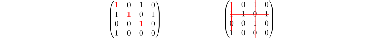
Now a related question: We want to draw as few lines as possible through rows and columns to cover up all the 1s in the matrix. An example using three lines is shown above on the right. This is as few lines as possible. Notice that the minimum number of lines needed is the same as the maximum collection size. This is a consequence of the König-Egerváry theorem. To see this, we can turn both matrix problems into bipartite matching problems as follows:

Create a bipartite graph where the vertices of X correspond to the rows of the matrix and the vertices of Y correspond to the columns of the matrix. Add an edge between vertices R_i of X and C_j of Y if and only if the matrix entry at row i, column j is 1. Shown below are the matching and covering on the graph that correspond to these matrix problems.

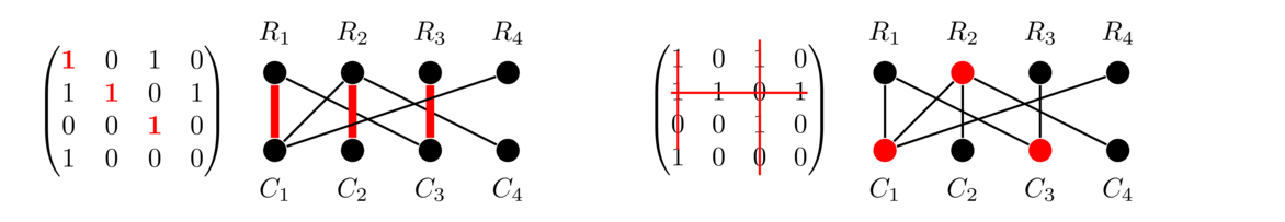
Matchings in this graph correspond to the problem of finding 1s in the matrix with no two 1s in the same row or column. If we include an edge from R_i to C_j, that corresponds to taking a 1 in row i, column j of the matrix. Because we are creating a matching, that means we cannot have any other edges incident on R_i or C_j, which is equivalent to saying we cannot take any other 1s in row i or column j. Similarly, coverings in this graph correspond to crossing out rows and columns of the matrix with lines.

Hall's theorem

We are often interested in perfect matchings, matchings where every vertex is matched. This requires both X and Y to be the same size. If Y happens to be bigger than X, then we are interested in matchings in which every vertex of X is matched. Here is one example of a graph where such a matching is impossible.

The problem is vertices a, b, and c only have edges to A and B. That is, we have three vertices of X that have to be matched to just two vertices of Y, so some vertex of X will have to be left out of any matching. In general, if something like this ever happens, where there is a collection S of vertices of X whose neighborhood (the set of all neighbors of vertices of S) is smaller than S, then there cannot be a matching that includes all of X. The surprising thing is that this is the only thing that we have to avoid. This result is called Hall's theorem.

(Hall's theorem) Consider a bipartite graph with partite sets X and Y. There is a matching that includes every vertex of X if and only if for every subset S of X, the size of the neighborhood of S is at least as large as the size of S.

First, if there is some subset S of X whose size is larger than the size of its neighborhood, then in any matching, some vertex of S will be left out.

Now assume there is no such subset. We will use the König-Egerváry theorem. Let C be a minimum vertex cover, and let C_X and C_Y denote the parts of C in X and Y, respectively. Let S be X-C_X, all the vertices of X that are not part of the covering. Since they are not part of the covering, any edge with an endpoint in S must be covered by a vertex of C_Y. So the neighbors of S must all lie in C_Y. Thus, by the hypothesis of the theorem, |C_Y| ≥ |S|. Thus we have β = |C_X|+|C_Y| ≥ |C_X| + |S| = |X|. So the minimum covering is at least as large as the size of X, meaning the maximum matching is that large as well, by the König-Egerváry theorem. Since this is a bipartite graph and at least |X| vertices are matched, then every vertex of X must be matched.

See the figure below for an overview of what is happening.

TONCAS

This theorem is an example of what some graph theorists call TONCAS: “The Obvious Necessary Condition is Also Sufficient.” That is, there is something that very clearly needs to be true for the thing in question to work, and that turns out to be the only thing that needs to be true. For Hall's theorem, in order to match everything in X, we must have every subset S of X have at least as large a neighborhood as there are things in S (the obvious necessary condition). And this is the only thing that needs to be true in order to match everything in X (the condition is also sufficient).

We have seen this before with the even vertex condition for Eulerian circuits. After looking at the Königsburg Bridge Problem, we quickly concluded that odd vertices prevent Eulerian circuits (the obvious necessary condition), and the surprising (and harder to prove) fact, is that this condition is also sufficient, that if there are no odd vertices then there is an Eulerian circuit. There are many more examples throughout graph theory.

Equivalency of Hall's theorem and the König-Egerváry theorem

There is also an interesting connection between Hall's theorem and the König-Egerváry theorem. Not only can we use the König-Egerváry theorem to prove Hall's theorem, but it is also possible to go the other way—namely, we can prove Hall's theorem from scratch and then use Hall's theorem to prove the König-Egerváry theorem. So, in some sense, the theorems are equivalent. There are a few other theorems like Menger's theorem and the max-flow min-cut theorem that we will see later that are equivalent to Hall's theorem and the König-Egerváry theorem in the same way. So there is some deeper underlying principle that manifests itself in different ways throughout graph theory.

Marriage theorem

Hall's theorem is sometimes formulated as Hall's marriage theorem. The setup is we have an equal number of men and women. As a bipartite graph, the men form one set and the women form the other. There is an edge between a man and a woman if and only if they are compatible, and we want a perfect matching, so that each person is married to someone they are compatible with. Such a matching is possible provided for any subset of the men, their are at least as many women that they are collectively compatible with as there are men in the subset.

Systems of distinct representatives

Hall's theorem is often stated in the context of something called a system of distinct representatives. Here we have a collection of sets and we want to choose one element from each set to represent that set, with no element representing more than one set.

For example, in the collection of sets below on the left, an SDR is highlighted.

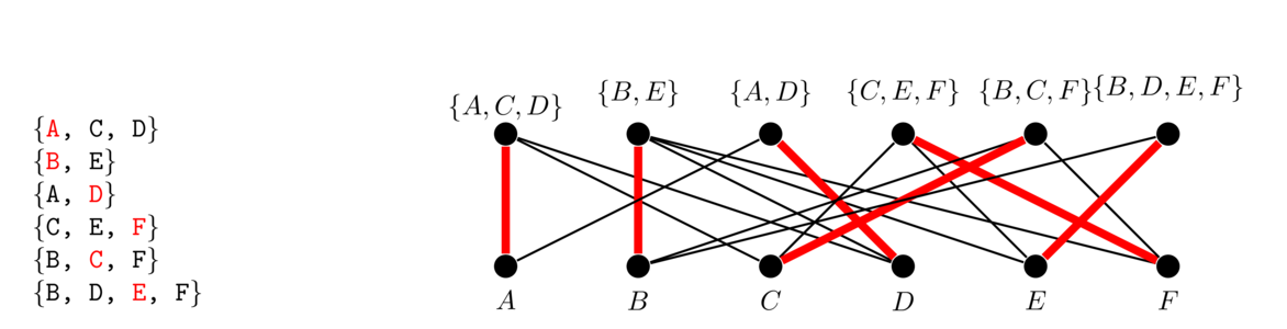
To relate this back to bipartite graphs, the partite set X consists of all the sets, the partite set Y consists of all the individual elements, and edges indicate if an element belongs to a set. See the graph above on the right for an example. Hall's theorem can be rephrased in terms of SDRs as follows: there exists an SDR for a collection of sets S₁, S₂, … S_n if and only if |S₁ ∪ S₂ ∪ … ∪ S_k| ≥ k for each integer k = 1, 2, … n.

As a somewhat practical example, perhaps the sets are committees of people and we want one person to represent each committee, with no one representing more than one committee.

Weighted bipartite matching

Consider the following problem: We have three people, A, B, and C, and three jobs a, b, and c. There is a certain cost associated with each person doing a given job. These costs are shown in the table below.

	a	b	c
A	2	4	1
B	3	2	6
C	8	4	7

We want to assign one job to each person, keeping the total cost to a minimum. This is typically called the assignment problem. We can represent the problem with a weighted bipartite graph, like below, where the people form one partite set, the jobs the other, and the costs becomes weights.

Since this problem is so small, we can quickly identify the optimal solution is to assign c to A, a to B and b to C for a total cost of 1+3+4 = 8. But for larger problems we would like a more systematic approach.

One way to do this problem would be to a greedy algorithm. Start by assigning person A the cheapest job for them, which would be c at a cost of 1. Then assign B the cheapest remaining job, which would be b at a cost of 2. But, this leaves C with job a at a cost of 8, which is not ideal. In general, a greedy approach for the assignment problem will work quickly but not produce optimal solutions.

There is a nice algorithm, called the Hungarian algorithm that can be used to find an optimal assignment. Assume that we have an n × n matrix of costs. The basic idea is we will manipulate the matrix in order to find a transversal, a collection of n zeros, no two of which are in the same row or column (this is similar to the matrix interpretation of the König-Egerváry theorem). The entries of the original matrix corresponding to the locations of the zeros in the transversal are the optimal costs. Here are the steps of the algorithm:

Subtract the smallest entry in each row from every entry in that row. If there is a transversal after doing this, then stop.
Subtract the smallest entry in each column from each entry in that column. If there is a transversal after doing this, then stop.
Draw lines through rows and columns to cover all the zeros. Find smallest uncovered entry, subtract that value from every uncovered entry, and add that value to all entries that are double-covered. If there is a transversal after doing this, then stop. Otherwise repeat this step as many times as needed.

In step 3, it is desirable, but not always necessary, to use as few lines as possible.

Let's try this algorithm on the example above. Start by subtracting the smallest entry from each row to get the table in the middle below. Then subtract the smallest entry from each column. This adds two additional zeros, which is enough for us to be able to find a transversal.

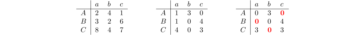
The optimal matching is Ac, Ba, Cb, with a total cost of 1+3+4 = 8, which comes from the original matrix.

Here is another example. The starting matrix of costs is on the left. First we subtract the smallest entry in each row from everything in its row. This gives the middle matrix. Then we subtract the smallest entry in each column from everything in its column. This gives the right matrix.

After these steps, there is no transversal. We can cover all the zeros with three lines, as shown below on the left. The smallest uncovered entry is 1. We subtract that value from all the uncovered entries and add it to all the doubled covered entries (just the last two entries in row 2). This gives the matrix in the middle from which we can find the transversal highlighted on the right.

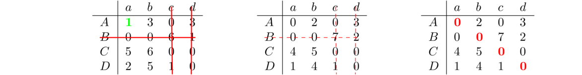
The optimal assignment is Aa, Bb, Cc, Dd, for a total cost of 2+4+1+1 = 8.

Why the algorithm works

The key idea is that if we add a value (positive or negative) to all things in a row or to all things in a column, it has no effect on the optimal assignment. The reason is that doing so has no effect on the relative costs. So steps 1 and 2 do not affect the optimal assignment. Step 3 seems like it might, but it is actually equivalent to this: Let m be the minimum uncovered entry. Add m to all covered rows, add it to all covered columns, and subtract it from every entry in the matrix. This is just a repeated application of adding a value to a row or column, so there is no net effect on the optimal assignment.

It still remains to be seen that the algorithm doesn't get stuck running forever. However, step 3 has the effect of bringing down the costs in the matrix at each step, so eventually we will have enough zeros to get a transversal.

Notes

The algorithm requires the matrix to be square. In other words, it requires an equal number of people as jobs. If the matrix is not square, to make it square we can add dummy rows or columns that consist of large values (any value larger than anything else in the matrix is fine). Here is an example:
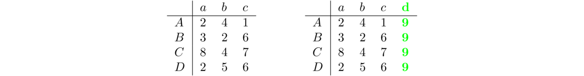
The person matched to one of the dummy jobs just doesn't get a job.
What if we want to maximize costs instead of minimize them? The solution is to take every entry in the matrix and subtract it from the largest entry in the matrix. For example, in the matrix below, subtract each entry from 8, the largest entry in the matrix.

Stable matching

In this section, we present the Gale-Shapley algorithm for stable matchings, an algorithm important enough that it helped lead to a Nobel Prize in economics for one of its creators. It is usually stated in terms of marrying people, though it has many applications, for instance in matching medical students to hospital internships.

We have an equal number of men and women. Each man has a list ranking the women in order of preference and each woman has a similar list ranking each man. We want to match the men to the women in a way that is stable. We never want it to happen that there is some man x and some women y who are not matched with each other but who prefer each other to the people they are matched with. If this ever happens, they would leave their current partners for each other. A matching in which this does not happen is called a stable matching.

First, here is the rough idea of how the algorithm works. We start with any man. That man proposes to the first woman on his list and they become engaged. Then at each stage throughout the process, we pick any man x who is not currently engaged. That man proposes to the first woman on his list whom he hasn't already asked. If that woman is free, then they become engaged. If that woman is currently engaged but prefers x to her current partner, then she leaves her current partner and becomes engaged to x. Otherwise, she rejects x. This process continues until everyone is engaged.

Here is a pseudocode description of the algorithm. The inputs are the sets X and Y of men and women along with each person's list of preferences.

while there is an x in X that is free
    pick an x from X that is free
    let y be the first choice on x's list
    remove y from x's list
    if y is free
        match x and y
    if y is matched and prefers x to her current partner
        match x and y
        send y's old partner back to being free

Suppose the men are named a, b, c, and d, and the women are named w, x, y, z. Here are the preference lists:

a :	wxzy	w :	bacd
b :	wzxy	x :	adcb
c :	wyxz	y :	badc
d :	wxyz	z :	cdba

Initially, everyone is free. Whenever we have a choice of which free man proposes next, we will go alphabetically. Here are the steps the algorithm takes.

Step	Action	Matching
1	a proposes to his first choice, w, and they become engaged.	aw
2	b proposes to his first choice, w. She prefers b to her current partner, so b and w become engaged, and a is now free	bw
3	a, now being free, proposes to the next choice on his list, x, and they become engaged.	ax, bw
4	c proposes to w and is rejected.	ax, bw
5	c then proposes to y who is free, so c and y become engaged	ax, bw, cy
6	d proposes to w and is rejected.	ax, bw, cy
7	d proposes to x and is rejected.	ax, bw, cy
8	d proposes to y. She prefers d to her current partner, c, so she drops c and becomes engaged to d	ax, bw, dy
9	c proposes to x and is rejected.	ax, bw, dy
10	c proposes to z and they become engaged.	ax, bw, cz, dy

Note that the resulting matching is stable. The pair bw is stable since they both have their first choice. Then looking at ax, a is x's first choice, while a's first choice is w, but she is already locked in with b. So ax is stable. Next in the pair dy, both d and y have their third choices, but as all of their preferred partners are locked up, neither d nor y could switch with anyone. Finally, in the pair cz, z has her first choice, but c has his last choice. However, c has no chance with any of the other women, so this pairing is stable.

Notes

We have presented this algorithm going through a single proposal at a time. Sometimes you will see it presented in terms of rounds where each free man proposes at once, and each woman chooses her favorite proposal from among them (sticking with her current partner if none of the proposals is better). This process produces the same stable matching as the one we have presented.
It should be noted that the algorithm as presented is man-optimal. Each man is married to the highest ranked woman on his list that is allowed under a stable matching. But the women are not necessarily as lucky. For the women, each woman is married to the lowest ranked man possible in any stable matching. Notice that each successive engagement moves down a man's preference list. Each time a man is engaged to someone new, it is someone farther down his list. Conversely, each successive engagement moves up a women's preference list. Each time a woman is engaged to someone new, it is someone farther up her list.
This actually occurred with the medical students/hospitals problem, where initially the hospitals were the ones doing the proposing and it was later changed so that the medical students did the proposing.

Why does it work?

First, is everyone matched? All of the men are matched since every woman appears on every man's list, and the algorithm says that any unmatched woman must accept a proposal. If there are the same number of women as men, then all of the women are matched as well.

Next, is the algorithm guaranteed to stop? The answer is yes because at each stage we remove a woman from a man's list, which means the men's preference lists are continually decreasing in size. If there are n men and n women, then there a total of n² entries, giving a worst case scenario of n² steps.

Next, are the matchings stable? Suppose they were not. In particular, suppose man p and woman q prefer each other to their current partners q' and p'. Since p prefers q to q', he must have proposed to q before q'. There are two possibilities. First, it is possible that q rejected p because she was matched to someone she preferred more. But if that was the case, she could not have ended up with p', whom she prefers less. Second, it is possible that p and q became engaged when p first proposed and then q later dumped him. But then she would have dumped him for someone she prefers more, and could never have ended up with p'.

More about matching

Matchings in general graphs

The results on matchings for bipartite graphs can be extended to work for general graphs. Odd cycles can cause problems for the augmenting path algorithm; however, there is an extension, called the Edmonds blossom algorithm, that is able to work around these problems. We omit the details here.

Hall's theorem has an analog for general graphs, known as Tutte's theorem. Here is the key idea behind it: Suppose we remove a subset S of vertices and look at components of remaining graph. If any component has an odd number of vertices then at least one of its vertices must be matched with something from S. Why? If the component has an odd number of vertices, we can't have the matching totally contained within that component, so some vertex must be matched with something outside, and that can only be something in S. Each such component with an odd number of vertices uses up a vertex from S, so we can never have more of them than vertices of S. Tutte proved that this obvious necessary condition is also sufficient:

(Tutte's theorem) A graph G has a perfect matching if and only if for every subset S of its vertices, the number of components of G-S with an odd number of vertices cannot exceed the number of elements of S.

The sufficiency part of the proof is a little involved, and we will not include it here. Notice the similarity of the statement with the statement of Hall's theorem.

Factoring graphs

Perfect matchings can be generalized to the concept of factors. Usually when we refer to a matching, we just think about edges. If we include the vertices of each edge in a matching, we get a subgraph, and that subgraph is 1-regular and includes every vertex in the graph, provided the matching is perfect. This leads to the following definition: A k-factor in a graph is a k-regular subgraph that includes every vertex of the graph. An example one-factor is shown below.

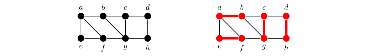
Since the only 2-regular graphs are cycles, a 2-factor is a collection of cycles in the graph that collectively use all the vertices exactly once. An example is shown below.

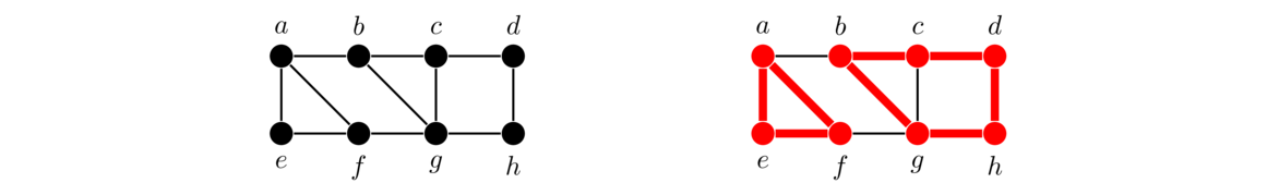
From here, we can talk about a graph being k-factorable if we can break it up into k-factors such that every edge of the graph is part of exactly one of the factors. Remember that each factor must use every vertex of the graph. Below are 1-factorings of K₄ and K_3,3.

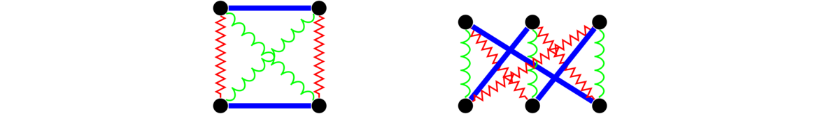
These figures were taken directly from the section on edge coloring. Recall from that section that matchings were the key to edge coloring bipartite and complete graphs.

Shown below on the left is a 2-factoring of a the graph C₈² (the cycle C₈ along with edges added between any vertices that are two steps apart on the cycle). On the right is a 2-factoring of K₇.

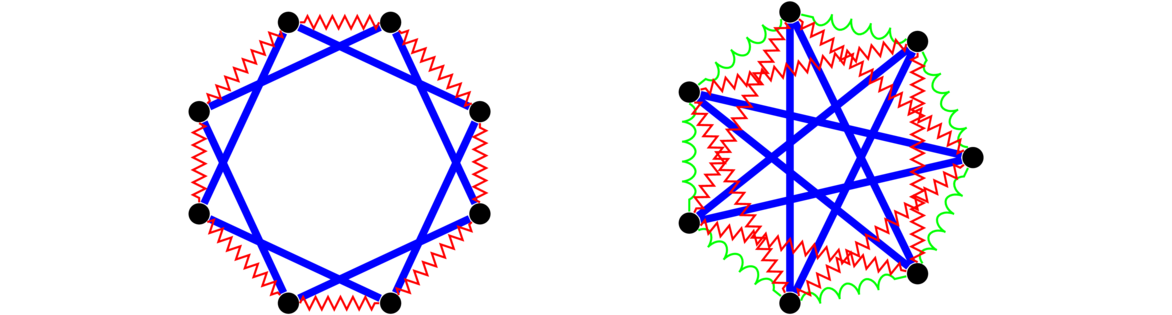
It is not to hard to show that all complete graphs with an even number of vertices are 1-factorable. Also, any k-regular bipartite graph with k ≥ 1 is 1-factorable. There is a nice theorem about 2-factors, first proved by Julius Petersen (the same guy that the graph is named for) that a graph is 2-factorable if and only it is regular with all vertex degrees being even. Finally, people have generalized this idea of factoring even further, looking at factoring a graph into copies of other graphs, like factoring a graph into triangles.

Digraphs

Definitions and properties

It is often useful to add a notion of direction to the edges of a graph. This gives us the concept of a directed graph, or digraph for short. An example is shown below.

A natural use for digraphs is in modeling road networks. An undirected graph can only model two-way roads, but a directed graph gives us the ability to model one-way roads. If our road network has a mix of one-way and two-way roads, we can use a pair of directed edges, one in each direction, for the two-way roads.

As another example, graphs are often used to model the states in a game. The states are the vertices and edges between vertices indicate that it is possible to go from one state to the next in the game. In many games, moves are one-way only, like in checkers or chess, so a directed graph would be more appropriate than an undirected graph for modeling states of many games.

Back in Chapter 1, we defined the edges of a graph to be two-element subsets of vertices. In a directed graph, instead of subsets, we use ordered pairs for edges. Here is the formal definition.

A directed graph, also called a digraph, is a pair (V,E), where V is a set of objects called vertices and E is a collection of ordered pairs of elements of V, called directed edges (or sometimes just edges).

We will usually write a directed edge from u to v as u → v. The vertex u is called the head and v is called the tail. We can also create multidigraphs, where loops and multiple edges are allowed.

The notion of degree of a vertex is now split into two notions: the indegree and outdegree. The indegree of a vertex v is the total number of edges directed from other vertices into v and the outdegree is the total number of edges directed from v to other vertices.

A few simple theorems about digraphs

One of the first theorems we looked at was the Degree sum formula, that says that the sum of the vertex degrees in a graph is twice the number of edges. It has a natural analog for digraphs.

(Degree sum formula for digraphs) In any digraph, the sum of the indegrees of all the vertices is equal to the number of edges in the digraph. Similarly, the sum of the outdegrees of all the vertices is equal to the number of edges in the digraph.

Every edge has a head and a tail. The head contributes 1 to the sum of the outdegrees, while the tail contributes 1 to the sum of the indegrees.

The even-degree theorem about Eulerian graphs also has a nice digraph analog. Recall that a graph has an Eulerian circuit if and only if every vertex has even degree. Here is the digraph version. It uses the term strongly connected, which will be defined a little later.

A strongly connected digraph has an Eulerian circuit if and only if the indegree of every vertex matches its outdegree.

Representing digraphs

In Section 2.3, we had an adjacency list representation of a graph. Here is the equivalent for a digraph.

class Digraph(dict):
    def add(self, v):
        if v not in self:
            self[v] = []

    def add_edge(self, u, v):
        self[u].append(v)

If you look at the original, you'll see that it this digraph class is exactly the same, except it does not have the line self[v].append(u) in the add_edge method. That is what makes the edges two-way in an ordinary graph. Leave it out and we have a one-way edge.

A little more vocabulary

Here are a few more important terms.

We will sometimes refer to directed paths and directed cycles in a digraph. These are paths and cycles that respect the orientations of the edges. For example, highlighted below are a directed path, abcdh, and a directed cycle, abcgfea. Notice that in both cases, the edges all go in the same direction as you trace along the path and as you trace along the cycle.
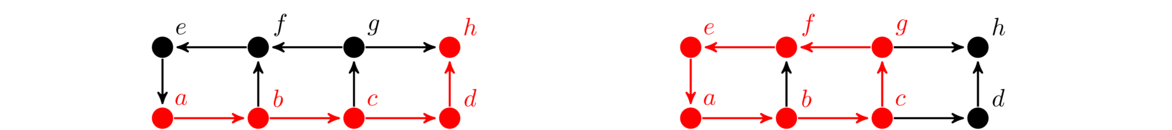
We may sometimes refer to the underlying graph of a digraph. This is the graph obtained from a digraph by removing all the directions from the edges.
One way to construct a digraph is to take an ordinary graph and add directions to its edges. This is called an orientation of a graph.

Connectedness of digraphs

The notion of connectivity in digraphs is more subtle than it is for ordinary graphs. Recall that a graph is connected if it is possible to get from any vertex to any other via a path. In a digraph it may happen that the underlying graph is connected, but because of the way the edges are oriented, it might not be possible to get from one vertex to another. This leads to two types of connectivity in digraphs.

A digraph is weakly connected if its underlying graph is connected. A digraph is strongly connected if there is a directed path between any two vertices in the digraph.

See the figure below for three digraphs. The left one is not connected at all. The middle one is weakly connected, as its underlying graph is connected, but when we account for directions, there is no way to get from the top vertex to any other vertex. The rightmost graph is strongly connected as we can follow directed edges to get from any vertex to any other.

Strong components

We are often interested in the strong components of a digraph, which are the digraph equivalent of components in an ordinary graph. They are defined as follows:

A strong component of a digraph is a maximal strongly connected subgraph.

This means two things:

Within a strong component, there is a directed path from every vertex to every other vertex.
A strong component is as large as possible in that you could not add any other vertices to it and still have it be strongly connected.

For example, in the digraph below, the subgraph induced by a, b, f, and e is one strong component, and the subgraph induced by c, d, h, and g is another. Notice that you can get from any vertex to any other within each component. Notice also that these components are as large as possible. If we were to add any vertices to either, it would no longer be possible to get from every vertex to every other one in the component.

Strong components are useful in a number of contexts. For example, we could have a graph that represents relationships between people, with an edge from one person to another if that person knows the other person's contact info. In a strong component of such a graph, if we give a message to any one person, that message could then get to any other person in that component.

Strong components can be found by using a slightly more sophisticated version of the depth-first search approach we took in Section 2.4. In particular, one simple approach, called Kosaraju's algorithm, involves performing two depth-first searches, one on the digraph and one on the digraph with its edges reversed. We omit the details here.

Orientations

It is interesting to ask when it is possible to orient the edges of a graph to create a strongly connected graph. A cut edge would prevent us from doing this as we can orient that edge in only one direction and that would make it impossible to get from anything on the tail side of the cut edge to anything on the head side. See below for an example.

This is a necessary condition, and it turns out to also be sufficient. We can strongly orient any connected graph that has no cut edge.

There exists an orientation of a connected graph that creates a strongly connected digraph if and only if the graph contains no cut edges.

As mentioned above, a cut edge prevents such an orientation. Assume the graph has no cut edge. Theorem 6 tells us an edge is a cut edge if and only if it is not on a cycle, so every edge lies on a cycle.

Start by taking any cycle C in the graph and orienting it so all edges point in the same direction along the cycle. If C includes every vertex, then we're done. Otherwise, find some vertex v that is not on C but is adjacent to a vertex u on C. We know v exists since the graph is connected. The edge uv must be part of some cycle D. Starting at v, we trace along D, orienting its edges to all point in the same direction until we reach a vertex on D, which could be u or something else. Notice that it is now possible to get from any vertex on C ∪ D to any other by tracing along C and D. From here we continue this process by finding another vertex w that is not on C or C but is adjacent to a vertex of C ∪ D. It is part of a cycle, E and we trace along E, orienting edges consistently in the same direction until we reach a vertex of C ∪ D. Continuing adding things this way until all vertices are accounted for. Any remaining edges can be oriented in whatever way we like.

See the figure below for how the first few steps of the proof work. What the proof creates is sometimes called an ear decomposition of the graph, because at each step it looks like we are adding a little ear to what we have built up thus far.

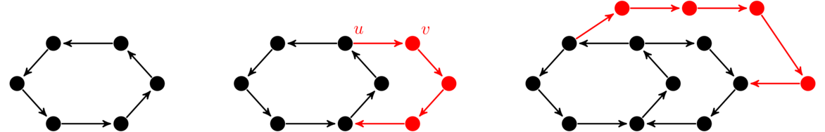
Directed acyclic graphs

One particularly important class of directed graphs are directed acyclic graphs, or DAGs. These are digraphs that contains no directed cycles; they are basically the digraph equivalent of forests. The underlying graph of a DAG might not look like a tree or forest, like the one shown below on the left, but when we take into account orientations, it behaves just like one.

The key property of DAGs is that we can order their vertices in such a way that there is never an edge directed from a vertex later in the ordering back to a vertex earlier in the ordering. For example, in the graph above on the left, if we arrange its vertices in the order e, f, g, d, a, b, c, as shown on the right. We see that edges are always directed from left to right. This type of ordering is called a topological ordering.

This is important, for example, in scheduling. We often want to know which tasks need to be done before which other tasks. In a DAG, we know that we can order the tasks so that a task's prerequisites are always completed before the task itself.

There is nice algorithm that finds this ordering, called a topological sort. Here is the basic idea: a vertex that has indegree 0 only has edges out from it. Therefore, it can safely go at the beginning of the ordering. Then delete that vertex (and all of its edges) and find another vertex of indegree 0. Put that vertex next in the order, delete it, and repeat until all vertices have been ordered. Here are the first three steps of the algorithm on the DAG above.

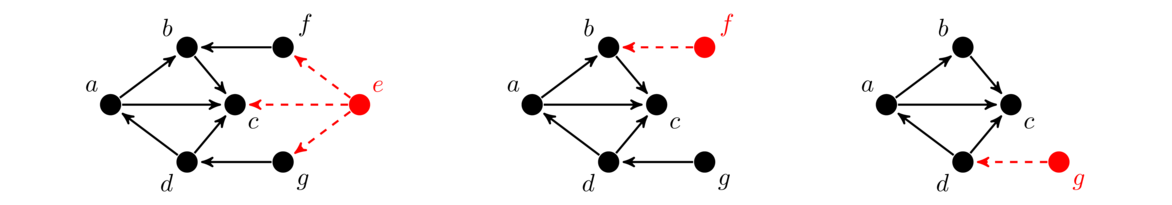
After this, d, a, b, and c are removed, in that order, giving us a topological ordering of e, f, g, d, a, b, c. Note that if there are multiple vertices of indegree 0, we can pick any one of them. There can be many possible topological orderings.

Will this always work? Since at every stage we choose a vertex v of indegree 0 in the graph that remains, we are guaranteed that no vertices that come later in the order can have edges directed backwards toward v. But then the main problem would seem to be that there might be no vertex of indegree 0 available. However, this is not the case. A DAG must always have a vertex of indegree 0.

To see why, suppose there were no vertices of indegree 0. Start at any vertex v₁. It has indegree greater than 0, so there must be some edge v₂ → v₁. Similarly v₂ has indegree greater than 0, so there is some edge v₃ → v₂. We can keep doing this, but since the digraph has a finite number of vertices, we must eventually reach a vertex we have already reached, creating a directed cycle. But this a directed acyclic graph, so there can't be any cycles, and we have a contradiction. Note also that removing vertices from a DAG can't add any cycles, so at every step of the topological sort we are working with a DAG.

Finally, note that we could also find a topological ordering in the reverse way, by successively removing vertices of outdegree 0.

Tournaments

A tournament is an orientation of a complete graph. It is called a tournament because it serves as a digraph model of a round-robin tournament where every team plays every other team exactly once. An edge v → w indicates that team v beat team w. An example is shown below.

On the right, we've drawn a linear representation of the tournament where only “upsets” are shown. Any edge that is not shown is assumed to go from left to right. Though we will not cover it here, it is an interesting problem to find an ordering in a tournament that minimizes the number of upset edges.

A king in a tournament is a vertex x such for every vertex v, either x beats v or x beats another vertex that beats v. The following fact might be a little surprising.

Every tournament has a king.

Take any vertex x of maximum outdegree. That vertex is a king. To show this, we just have to show that if there is any vertex v that x does not beat, then x does beat another vertex that itself beats v. If there were no such vertex, then v would beat every vertex that x beat, giving v a higher outdegree than x (since v also beats x). This is impossible since x has maximum outdegree, so there must be such a vertex, meaning that x is a king.

Here is another fact that might be a little surprising.

Every tournament has a Hamiltonian path.

Let P = v₁v₂… v_k be a maximum length path in the graph. Suppose there is some vertex w that is not on the path. We know that w cannot beat v₁ as otherwise wv₁v₂… v_k would be a longer path than P. This then implies that w cannot beat v₂ as otherwise v₁wv₂… v_k would be a longer path than P. Similarly, w cannot beat v₃ as otherwise v₁v₂wv₃… v_k would be a longer path than P. Continuing in this way, we see that v_i beats w for each i = 1,2,…, k. But this leads to a contradiction because then v₁v₂… v_kw is a longer path than P. Thus there can be no vertex that does not lie on P, making it a Hamiltonian path.

The figure below might help in visualizing how the proof works.

Note, however, that a tournament need not have a Hamiltonian cycle, as the example below shows.

Note that the tournament above possesses a special property: it is transitive. That is, whenever x beats y and y beats z, then x beats z. Transitive tournaments have nice properties. In particular, they have no cycles, which makes them DAGs. Thus it is possible to order the players in a transitive tournament so that there is never an upset, where a lower ranked team beats a higher ranked team.

There is a whole lot more to tournaments (and digraphs in general). We have only scratched the surface.

Connectivity

Definitions and properties

Very early on, we defined connectivity in a graph to be the existence of a path from any vertex to any other. But some graphs are more connected than others. For instance, a tree is minimally connected, as removing any vertex or edge from a tree will disconnect it. On the other hand, a complete graph is very well connected. We want a way to measure the connectivity of a graph. The typical way this is done is to look at how many vertices or edges need to be deleted in order to disconnect the graph.

A graph is called k-connected if it takes the removal of at least k vertices in order to disconnect the graph. The connectivity of a noncomplete graph G, denoted κ(G), is the minimum number of vertices that need to be deleted in order to disconnect the graph.

A graph is called k-edge-connected if it takes the removal of at least k edges in order to disconnect the graph. The connectivity of a graph G, denoted κ'(G), is the minimum number of edges that need to be deleted in order to disconnect the graph.

The connectivity of the complete graph K_n is a special case. By convention, κ(K_n) = n-1.

Note the difference between connectivity k and k-connected. A graph with connectivity 3 is 1-connected, 2-connected, and 3-connected. The connectivity is tells us the maximum k for which a graph is k-connected. A disconnected graph has connectivity 0. A graph has connectivity 1 if and only if it has a cut vertex, and it has edge connectivity 1 if and only if it has a cut edge. A 2-connected graph has no cut vertex and a 2-edge connected graph has no cut edge. Here are a few examples of connectivity in graphs:

Recall that δ is notation for the minimum degree in a graph. We have the following theorem.

For any simple graph, κ ≤ κ' ≤ δ.

First, κ' ≤ δ since removing the edges incident on a vertex of minimum degree will disconnect the graph.

To show κ' ≤ κ, let E be a minimum size set of edges whose deletion breaks the graph into two components, S and T. So |E| = κ'. It might happen that E consists of every edge between S and T. If so, then E has a lot of edges, |S| · |T| in total, which is greater than n-1, and n-1 ≥ κ (where n is the number of vertices in the graph).

Otherwise, there exist s ∈ S and t ∈ T that are not adjacent. Consider the set consisting of all the neighbors of s in T and all the other vertices of S that have neighbors in T. Removing the vertices of this set will disconnect the graph as we will not be able to get from s to t. So this set has size at least κ. On the other hand, the edges between the two halves of this set come from E, so it has size no larger than κ', and so we get κ ≤ κ'.

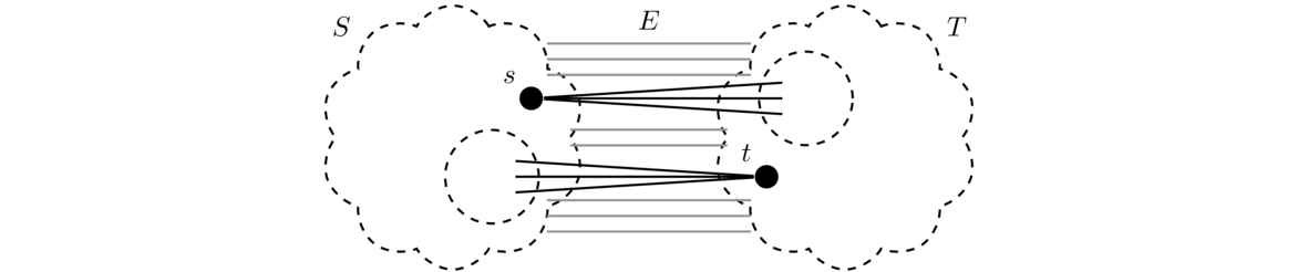
Blocks

Recall that a component of a graph is a maximally connected subgraph. If we replace “connected” with “2-connected”, we get the notion of a block.

A block in a graph is a maximal 2-connected subgraph of the graph.

That is, it is a subgraph that contains no cut vertices and adding any more vertices would introduce a cut vertex. Basically, we can break up a graph around its cut vertices into blocks, like in the figure below.

This is somewhat reminiscent of how a graph breaks into components, except instead of breaking the graph into maximal connected pieces, we are breaking it into maximal 2-connected pieces. The reason this is important is that many graph problems can be simplified by reducing a graph into blocks.

For example, the chromatic number of a graph is the maximum of the chromatic numbers of its blocks. In the graph above the chromatic number is 3 since the triangle block requires 3 colors, while the others require 2. As another example, the number of spanning trees in a graph is the product of the number of spanning trees in each block. As one further example, planarity can be reduced to blocks: a graph is planar if and only if each of its blocks are planar.

Menger's theorem

We come to a famous result in graph theory, known as Menger's theorem. We are given two vertices in a graph and we want know how many vertices we would have to delete in order to separate the two vertices, i.e., make it impossible to get from one to the other. For example, in the graph below, we have to delete three vertices in order to make it impossible to get from s to t.

We are also interested in how many routes there are from s to t that don't share any vertices (besides s and t themselves). In the graph above, there are many routes from s to t, and we can find 3 routes that don't share any vertices—we can go across the top, across the bottom, or straight through the middle. Notice that this number, 3, is the same as the number of vertices we need to delete to separate s from t. This is no coincidence. It is an example of Menger's theorem.

(Menger's theorem) Let s and t be nonadjacent vertices in some graph. The minimum number of vertices that we would need to remove from the graph in order to make it impossible to get from s to t is equal to the maximum number of paths from s to t that share no vertices other than s and t.

Note that if we have a set of vertices that separates s from t, then that set must contain a vertex of every path between s and t, and if we are looking at disjoint paths from s to t, then no vertex can remove two paths at once. Thus the minimum number of vertices needed to separate s from t is at least as large as the maximum number of disjoint paths from s to t. Going the other direction, showing it is no larger, is quite a bit more involved, and we will skip it.

This is another minimax theorem, like the König-Egerváry theorem, where minimizing one quantity turns out to give the answer to the maximum of another. With the König-Egerváry theorem it was that a minimum vertex cover led to a maximum matching of the same size. Here a minimum separating set of vertices has the same size as the maximum number of vertex-disjoint paths. In fact, it is possible to use the König-Egerváry theorem to prove Menger's theorem and vice-versa. So these theorems are in some sense equivalent.

There is also an edge-version of Menger's theorem that states that the minimum number of edges that need to be deleted to separate s from t is equal to the maximum number of paths between s and t that share no edges. Finally, Menger's theorem leads to the following characterization of connectivity:

A graph is k-connected if and only if between any pair of vertices there are at least k paths that don't share any vertices besides their endpoints.

Network flow

The setup for network flow is we have a digraph and two special vertices, called the source and the sink. Each edge has a weight, called its capacity, and we are trying to push as much stuff through the digraph from the source to the sink as possible. This is called a flow, and the weighted digraph is called a network.

Shown below is an example. The source is a and the sink is h. The first number, highlighted in red on each edge, is the flow value, and the second number is the capacity. Note that the flow is not optimal, as it would be possible to push more stuff through the network than the current total of 6 units.

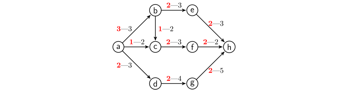
The amount of flow on an edge cannot exceed its capacity, and, except for the source and sink, the total amount of flow into a vertex must equal the total amount of flow out of that vertex. That is, the flow passes through the vertices, which neither create nor consume flow. The total amount of flow through the network is called the flow's value. That amount can be found by counting the total flow leaving the source or, equivalently, the total flow entering the sink.

Many real problems can be modeled by flow networks. For instance, suppose the source represents a place where we are mining raw materials that we need to get to a factory, which is the sink. The edges represent various routes that we can send the raw materials along, with the capacities being how much material we can ship along those routes. Assuming the transportation network is the limiting factor, we are interested in how much raw material can we get to the factory. Also, many seemingly unrelated graph theory problems can be converted into network flow problems. We'll see an example a little later.

Max-flow min-cut theorem

Closely related to flows are cuts. A cut is a set of edges whose deletion makes it impossible to get from the source to the sink. We are interested in the sum of the capacities of the edges in cuts. For example, shown below is a cut consisting of edges be, bc, ac, and dg. Its total capacity is 3+2+2+4 = 11.

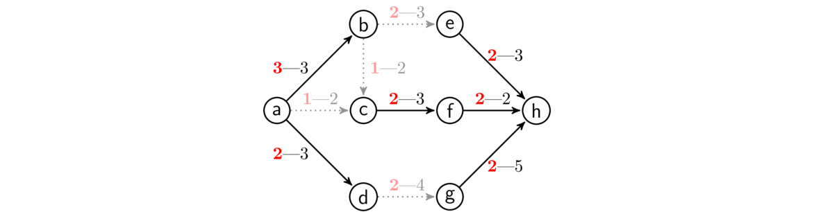
Notice the similarity between flows and cuts and what we were interested in with Menger's theorem—disjoint paths between vertices and sets that cut off the two vertices from each other. Below is an important relationship between flows and cuts in a network.

In any network, the value of every flow is less than or equal to the capacity of every cut.

Given any cut C, every flow must pass through at least one edge of C. If not, then C would not be a cut since there would be a way to get from the source to the sink along that flow. Since a flow must pass through at least some edges of C, its value cannot exceed the total capacities of those edges.

In particular, if we can find a flow and a cut of the same size, then we know that the our flow is a maximum flow (and that the cut is minimum as well). Notice the similarity between this theorem and Theorem 34, which relates matchings and covers. And we have the following theorem, the network analog of the König-Egerváry theorem:

(Max-flow min-cut) In any network, the maximum value of a flow equals the minimum value of a cut.

As an example, in the network below a maximum flow is shown. A total of 8 units of flow move through the network as can be seen by adding up the flow out of the source or the flow into the sink. A minimum cut in this network consists of the edges a → b, a → c, and a → d, whose total capacity is 3+2+3 = 8. Since we have a flow and a cut of the same size, our flow is maximum and our cut is minimum.

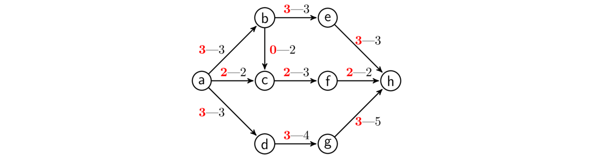
The hard part of the proof of this theorem is showing that we can always find a flow with the same value as some cut. This can be done with an algorithm known as the Ford-Fulkerson algorithm, so named for its creators.

The Ford-Fulkerson algorithm

The basic idea of the Ford-Fulkerson algorithm is that it starts with a flow and uses it to find either a better flow or a minimum cut. It does this by looking for paths from the source to the sink along which to improve the flow. The simplest case of such a path is one where all the flow values are below capacity, like in the example below. The flow can be increased by one unit along the path highlighted, as shown on the right.

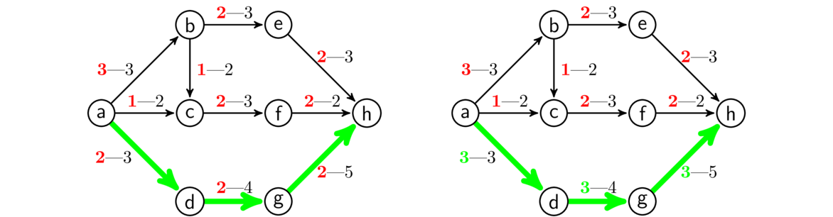
However, there is another case to consider: backward edges. In the example shown below, we have highlighted a path. Notice that the edge from b to c is backwards. We can steal a unit of flow from that edge and redirect it along the edge from b to e. This gives us a path that increases the flow, as shown on the right.

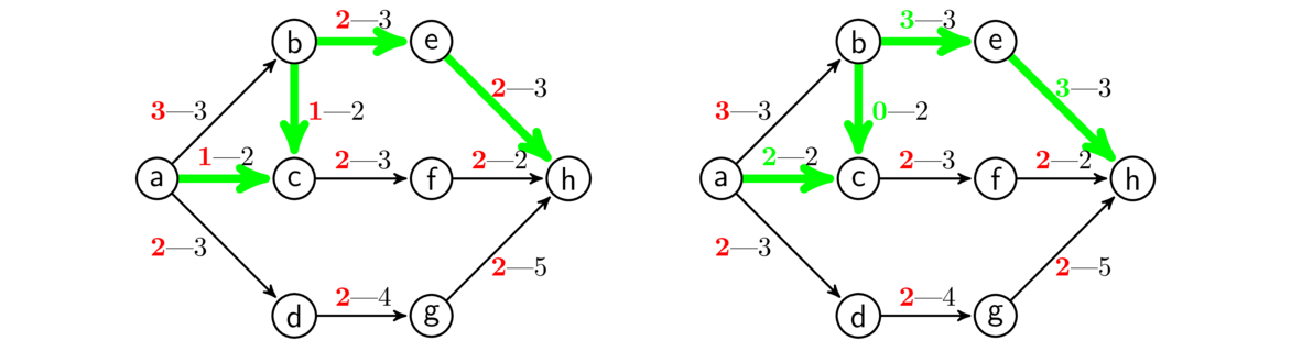
What happens is there are initially 3 units of flow entering vertex b, with 2 units heading to e and 1 unit heading to c. We redirect that one unit so that all 3 units go from b to e. This frees up some space at c, which allows us to move a new unit of flow from the source into c, which we can then send into f.

The Ford-Fulkerson algorithm starts with a flow of all zeroes on each edge and continually improves the flow by searching for paths of either of these two types until no such paths can be found. At the same time as it is doing this, it searches for cuts. It does this by maintaining two sets, R and S. The set R is all the “reached” vertices and the set S is all the “searched” vertices. Initially, R consists of only the source vertex and S is empty.

The algorithm continually searches paths on which to improve the flow as follows: It picks any vertex v of R-S and looks for edges v → u that are under capacity or edges u → v that have positive flow. Whenever it finds such an edge, it adds u to R. Once all the edges involving v are looked at, v is added to S.

If the sink is ever added to R, that means we have a path along which we can increase the flow. On the other hand, if it ever happens that R and S are equal, then there are no new vertices left to search from, so we stop and return our flow as a maximum flow, and we return a minimum cut which consists of all the edges from vertices in S to vertices not in S.

Here is the pseudocode for the algorithm.

set flow on each edge to 0
while True
    R  =  {source}
    S  =  {}
    while sink is not in R
        if R  =  =  S
            return flow and S
        pick any vertex v in R-S
        foreach u such that v->u is an edge
            if u is not in R and flow on v->u is under capacity
                add u to R
                record v as the parent of u
        foreach u such that u->v is an edge
            if u is not in R and flow on u->v is positive
                add u to R
                record u as the parent of v
        add v to S
    using the recorded parents, trace along the path,
    adding 1 to flow on forward edges and subtracting 1 along backward edges

Two notes are in order here:

We have chosen to start with a flow that is initially all 0. This is an easy way to start, but we can start instead with any flow and the algorithm will build on it to find a maximum flow.
We increase the flow by 1 unit at a time. A more sophisticated approach is to increase the flow by as many units as possible along our path. For instance, if we have a path of forward edges, where each flow value is under capacity by at least 5 units, then we could increase the flow on each edge by 5 units.

Examples

For the network we have been looking at throughout this section, let's look at just the final step of the algorithm, where it finds a minimum cut. Shown below is the optimal flow returned by the algorithm.

Once the flow gets to this point, the last step of the algorithm starts with R = {a} and S empty. The algorithm attempts to find paths to increase the flow by searching from a, but it finds none as all the edges from a are at capacity. It then adds a to S and sees that R = S. This stops the algorithm, and the minimum cut consists of all edges from S (which is just a) to vertices not in S, so it consist of edges a → b, a → c, and a → d. Both the flow and the cut have size 8.

Another example

Below is a longer example. The source is a and the sink is g. On the left is our initial flow of all zeroes.

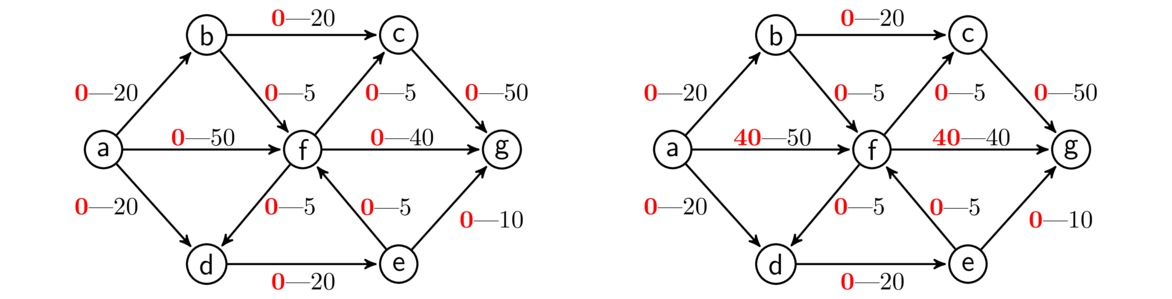
We start with R = {a} and S empty. We search from a and find the edges to b, d, and f under capacity. Thus we add b, f, and d to R, and having finished with a, we add it to S. We then pick anything in R-S, say b, and search from it. From there, we see edges to c and f under capacity, so we add those vertices to R (note that f is already there). Having finished with b, we add it to S, so at this point R is {a,b,f,d,c} and S is {a,b}. We then pick something else in R-S, say f, and search from it. There are some backward edges into f, but as none of those have positive flow, we ignore them. We have forward edges to c, g, and e, so we add them to R.

At this point, the sink, g, has been added to R, which means we have a path along which we can increase the flow, namely afg. Our algorithm keeps track of the fact that we reached f from a and that we reached g from f, and uses that to reconstruct the path. Then we can increase the flow by 1 along edges af and fg, or if we want to be more efficient, we an actually increase it by 40 units on both edges, as shown above on the right.

We then reset R to {a} and S to being empty and repeat the search. Several more searching steps follow until we arrive at the maximum flow shown below.

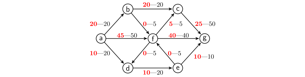
At the last step, we start again with R = {a} and S empty. The edges from a to f and d are below capacity, so we add them to R, and then we add a to S. Next, we pick something in R-S, say f. All of the new backward edges into f have 0 flow, and the only forward edge below capacity is to d, so we don't add anything new to R. So now R = {a,f,d}, S = {a,f}, and we explore from d. This adds only e to R. Exploring from e adds nothing new to R, and we end up with R and S both equal to {a,f,d,e}.

Since R = S, the algorithm ends, and our minimum cut consists of all the edges directed from vertices in S to vertices not in S, specifically edges ab, fc, fg, and eg, for a total capacity of 20+5+40+10 = 75, the same as the value of the flow.

More about network flows

The Max-flow min-cut theorem is the last of several big theorems we've met that are all equivalent to each other, the others being the König-Egerváry theorem, Hall's theorem, and Menger's theorem. There are still others, such as Dillworth's theorem and the von Neumann minimax theorem, that we haven't covered. They are equivalent to each other in the sense that each one can be used to prove any of the others.

Flows with multiple sources and sinks

It is not too hard to handle multiple sources and sinks. We create a single “super source” with edges directed towards every source and add infinite (or extremely high) capacity to each edge. A similar “super sink” can be added with edges of infinite capacity directed from every sink to the super sink.

Applications

The Max-flow min-cut theorem can be used for a variety of purposes. One can imagine various practical applications for shipping things from one location to another. There are also applications within graph theory as many problems can be transformed into network flow problems.

For instance, we can use network flow to find maximum matchings. Suppose we have a bipartite graph with partite sets X and Y. We can turn it into network flow problem as follows: Direct all edges of the bipartite graph from X to Y. Add a source vertex s with edges directed from s to every vertex of X. Add a sink vertex t with edges directed from every vertex of Y into t. Give every edge a capacity of 1. See the figure below.

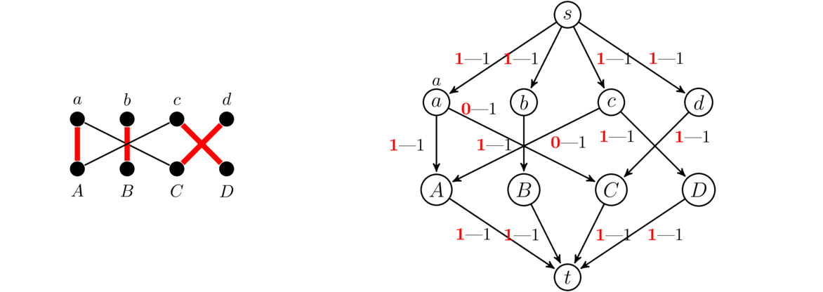
We then find a maximum flow and minimum cut in this network. A maximum matching is given by taking all the edges from X to Y that have a flow value of 1. The total value of the flow equals the size of the matching. All of the vertices of X and Y that belong to the minimum cut form a minimum vertex cover.

It is a nice exercise to run through the last step of the Ford-Fulkerson algorithm to find a minimum cut. A big part of this step consists of walking back and forth between X and Y along edges that alternately have flow 0 and flow 1 in a way that is exactly analogous to the bouncing back and forth between unmatched and matched edges that the augmenting path algorithm for matching does. In the end, we get S = {s, a, b, c, A, B}, giving us a minimum cut consisting of edges sd, At, and Bt. The three non-source and non-sink endpoints of these edges, d, A, and B form a minimum vertex cover. It's not too hard to formalize this in general to prove the König-Egerváry theorem.

Epilogue and Bibliography

If you've worked through all of the book, then you are familiar with most of the typical topics in graph theory. To really learn the material, be sure to try a lot of exercises. The material covered here is most of the contents of an ordinary graph theory class at an introductory level. You should have a foundation to learn more graph theory or to start applying graph theory to real problems.

If you're interested in learning more graph theory, see the books in the bibliography section that follows or look into some more advanced books. If you're interested in the algorithmic aspects of graph theory, most books on algorithms include a lot about graph algorithms.

Bibliography

Here is a list of books that I used in preparing these notes.

Introduction to Graph Theory, 2nd ed. by Douglas B. West, Prentice Hall, 2001 — This is the book I used in my graduate school introductory graph theory class. West covers a lot of material and does so very carefully. This is my goto reference if I forget something. West's exposition is maybe a little too efficient at times, making it a bit difficult for a beginning graph theory student, but it's definitely manageable, especially if you have a little bit of a background already in graph theory. His book contains a ton of really good exercises of all levels of difficulty.
Graph Theory: A Problem Oriented Approach by Daniel A. Marcus, Mathematical Association of America, 2008 — This a remarkable book. It is slender, inexpensive, and the author explains things very nicely. The “problem-oriented” approach means the book is full of interesting problems that help you learn the material by developing much of it yourself.
Introduction to Graph Theory by Gary Chartrand and Ping Zhang, Dover Publications, 2012 — This book is probably my favorite undergraduate graph theory textbook. It is well-organized and relatively short. It also contains a lot of historical information.
The Fascinating World of Graph Theory, Arthur Benjamin, Gary Chartrand, Ping Zhang — This book contains a lot of the same material as Chartrand and Zhang's book, but it is a different sort of book. It's a combination between a textbook and a popular math book for a general audience, so it contains a lot of prose, helping to explain and motivate the material. There really aren't enough math books like this one.
Graph Theory and Its Applications, 2nd ed. by Jonathan Gross and Jay Yellen, Chapman and Hall/CRC 2005 — This is another good textbook. I prefer the exposition of the authors listed above, but this is a great book if you are looking for lots of applications of graph theory. It also contains a number of algorithms that you won't find in most other books.

Exercises

The majority of these exercises are ones I made up myself, but there are a few I adapted that were inspired by ones from other books, in particular Introduction to Graph Theory, 2nd ed. by Douglas B. West, and Graph Theory: A Problem Oriented Approach by Daniel A. Marcus, and Introduction to Graph Theory by Gary Chartrand and Ping Zhang. See any of those, especially West's book, if you are looking for more challenging problems than the ones I have here.

Exercises for Chapter 1

Answer the questions about the graph below.
1. What vertices are adjacent to b?
2. The only perfectly horizontal edge is incident on what two vertices?
3. What is the degree of e?
Use the graph below on the left to answer the following questions.
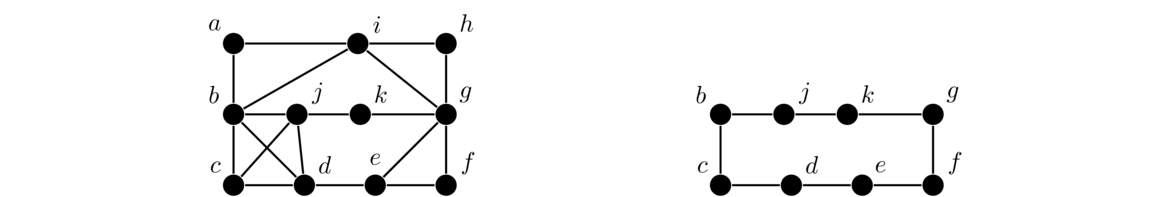
1. List the vertices of degree 2.
2. List the neighbors of b.
3. List the edges incident on a.
4. List all the cut vertices and cut edges (if any).
5. Find a 3-clique and a 4-clique.
6. Find an independent set containing 5 vertices.
7. Is the graph on the right above a subgraph of the graph on the left?
8. Is the graph on the right above an induced subgraph of the graph on the left?
Sketch the following graphs: P₇, C₇, and K₇.
Sketch a multigraph that has two vertices of degree 0, one vertex of degree 1, four vertices of degree 2, and one vertex of degree 3.
1. What graph covered in Chapter 1 is 3-regular and has exactly 10 vertices?.
2. Sketch a 3-regular simple graph that has exactly 12 vertices.
Sketch a single graph that has all of the following properties:
- has exactly 10 vertices
- connected
- has exactly 2 cut edges
- has a cut vertex that is not incident on a cut edge
- contains a 4-clique but no 5-clique
For the graph below find the following:
1. A subgraph that includes all the vertices except a and is not an induced subgraph.
2. A subgraph that includes all the vertices except a and is an induced subgraph.
1. Is P₅ an induced subgraph of C₆? Explain briefly.
2. Is P₆ an induced subgraph of C₆? Explain briefly.
Show that the two graphs below are isomorphic by giving a one-to-one correspondence.
Show the graphs below are not isomorphic by finding a property that one has that the other doesn't.
Three graphs are shown below.
1. Two of the graphs are isomorphic. Show this by giving a one-to-one correspondence between them.
2. One graph is not isomorphic to the other two. Explain why.
Use the graphs below to answer the questions that follow.
1. Sketch the line graph of A.
2. Show that A and B are isomorphic by explicitly giving the one-to-one correspondence.
3. Show that B and C are not isomorphic.
Let G = K₃ and H = P₄. Sketch G ∪ H, G∨ H, and G □ H.
Sketch C₅.
Sketch the following graphs:
1. K₄ ∪ P₄
2. P₃ ∨ C₃
3. G □ C₄, where G is the graph below on the left.
4. The line graph of the graph below on the right.
Let G and H be simple graphs with n₁ vertices and e₁ edges in G and n₂ and e₂ edges in H.
1. How many vertices and edges are there in G?
2. How many vertices and edges are there G □ H?
Fill in the blank:
1. A simple graph contains no or .
2. Every vertex of G has degree 3. Therefore G is a graph.
3. To prove that a graph is connected, it suffices to show that for any vertices u and v,
  .
True or False:
1. If a graph is connected, then every vertex is adjacent to every other vertex.
2. If a graph contains a vertex that is adjacent to every other vertex, then it is connected.
3. It is possible for every edge of a graph on 5 vertices to be a cut edge.
4. If edges e and f are incident on vertex u, then the vertices corresponding to e and f in the line graph must be adjacent.
Someone says a cut vertex is a vertex whose deletion breaks the graph into two components. What is wrong with this definition?
Find maximum-sized independent sets in these graphs. [Hint: the second answer has 8 vertices.]
Of all connected graphs with 10 vertices, which graph, if you remove just one vertex, breaks into the largest number of components? Draw it.
There are exactly 11 different simple graphs on 4 vertices (none of which is isomorphic to any other). Draw them.
Use set-builder notation to describe the vertex and edge sets of the following:
1. Wheel — The wheel W_n consists of a cycle C_n along with a central vertex adjacent to every vertex on the cycle.
2. Square of a Cycle — C_n² consists of a cycle along with extra edges added from each vertex to both vertices that are two steps from it along the cycle.
3. Grid — The grid G_n,m consists of vertices arranged in an n × m grid. [Hint: it might help to name the vertices with two subscripts.]
To help picture them, shown below are W₆, C₈², and G_3,4. Make sure your answers work for the general cases, not just these specific cases.

Exercises for Chapter 2

Note: For any of the programming problems in this chapter or others, it is recommended to use the Graph class from Section 2.3.

Sketch a graph containing 6 vertices whose degrees are 0, 1, 1, 2, 2, and 3, or explain why such a graph can't exist.
Explain why there cannot exist a graph on 10 vertices where the sum of the degrees of all the vertices is greater than 90.
Use the Degree sum formula to figure out how many edges there are in any k-regular graph on n vertices. Explain. [Note: the graph is k-regular, but not necessarily complete.]
A graph has 14 vertices and 27 edges. Of the vertices, 6 have degree 4 and the rest have degree 3 or 5. How many of each are there? Explain.
Suppose we have a simple graph with 8 vertices. It has one vertex of each of the degrees 1 through 7. What is the degree of the remaining vertex? Explain.
Can a disconnected graph be self-complementary (isomorphic to its own complement)? Explain.
Explain why the claw is not the line graph of any simple graph. The claw is a star with a central vertex and three outer vertices.
Consider the construction of regular graphs from Section 2.2 with n = 58 and k = 7. If we place the vertices around a circle and label them clockwise v₁, v₂, …, v₅₈, what are the names of the vertices that v₁ is adjacent to?
For all k ≥ 1, show how to construct a (2k+1)-regular multigraph that contains a cut edge.
Given n and k, describe how to create an n-vertex simple graph with an independent set of size k and as many edges as possible.
For the graph below, do the following:
1. Find its adjacency matrix representation.
2. Find its adjacency list representation.
3. Suppose both BFS and DFS are run on the graph, starting at vertex a and visiting all vertices in the graph. Assuming neighbors of a vertex are added in alphabetical order, indicate the order in which each of the two algorithms visits the vertices.
A decomposition of a graph is a list of subgraphs of that graph with each edge appearing in exactly one of those subgraphs. Essentially, you divide up the edges between different subgraphs, with no edge being used more than once. Color/line thickness can be used to illustrate it. For instance, shown below is a graph and a decomposition of it into copies of P₃.
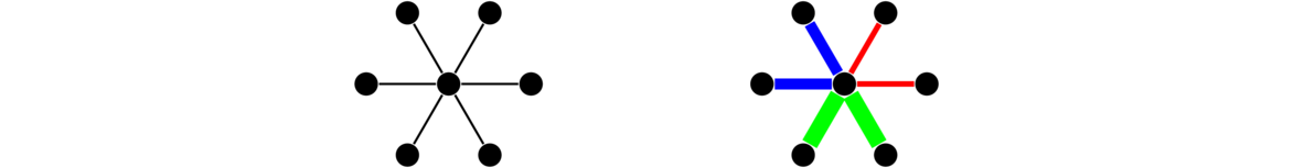
1. Show how to decompose K₅ into copies of C₅.
2. Show how to decompose the Petersen graph into copies of P₄.
Directly using the definition of connectedness, prove that the complete bipartite graph K_m,n is connected as long as m,n ≥ 1.
Suppose there are two vertices x₀ and y₀ in a graph G that are not adjacent to each other and that don't have a neighbor in common. Prove that in G, no vertex is at a distance of more than 3 from any other.
Prove that if every vertex in a graph is adjacent to at least half of the other vertices, then the graph must be connected.
Prove that if a graph contains two vertices that are at a distance of d from each other, then the graph must have an independent set with at least ceiling( (1+d)/2) vertices.
Prove if every vertex in a graph has degree at least d, then the graph contains a path at least d vertices long.
Prove that each endpoint of the longest path in a graph must have a degree that is no larger than the length of that path.
Write a program that creates a regular graph with n = 2000 vertices with each vertex having degree k = 31.
Program a function num_edges(G) that returns how many edges are in the graph G.
Program a function create_graph(V, E). It takes two strings and creates a new graph from them. For this problem, the names of the vertices in the graph will all be one character strings. The parameter V contains all the vertex names and the parameter E contains all the edge names, which consist of pairs of vertices separated by spaces. The function should read those strings, add vertices and edges to the graph based on them, and return the created graph. For instance create_graph("abcd", "ab ac bd") should build and return the graph with vertices a, b, c, and d and edges ab, ac and bd.
Program a function add_edges(G) that will allow us to add a bunch of edges to a graph in one line. The function has two parameters, a graph G whose vertices are one-character strings and a string s of edges separated by spaces. The method adds edges to G for each edge name in s. For instance, if s = "ab ac bc", this method will add edges from a to b from a to c and from b to c.
Modify the depth-first search algorithm to create a function has_cycle(G) that determines if the graph G has a cycle. [Hint: if depth-first search encounters a vertex that it has already seen, that indicates that there is a cycle in the graph. Just be careful that that vertex doesn't happen to be the parent of the vertex currently being checked.]

Exercises for Chapter 3

Is this the adjacency matrix of a bipartite graph? Explain briefly.
0 1 0 0 1 0
1 0 1 0 0 0
0 1 0 1 0 0
0 0 1 0 1 0
1 0 0 1 0 1
0 0 0 0 1 0
Construct a bipartite graph with 8 vertices that has as many edges as possible.
Show that the Petersen graph is not bipartite.
Show that the hypercube Q₄ is bipartite.
If you remove enough vertices from any graph, eventually you'll end up with a bipartite graph. What is the minimum number of vertices that need to be removed from the graph below to make the remaining graph bipartite? Which vertices in particular do you remove?
Suppose G is bipartite. Show that the line graph of G is not necessarily bipartite by giving a counterexample.
Sketch a 3-regular bipartite graph that is not a complete bipartite graph.
What is the maximum possible number of edges in a simple bipartite graph on n vertices? Explain.
True/False.
1. It is possible for there to be multiple paths connecting the same two vertices in a tree.
2. The point of Prüfer codes is that there is a one-to-one correspondence between them and labeled trees, which allows us to count how many spanning trees K_n has.
The degrees of the 10 vertices in a simple graph are 4,4,7,7,7,7,8,8,8,8. Give two different reasons why this graph cannot be a tree.
Is the graph below a tree? Explain.
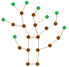
Use the formula τ(G) = τ(G-e)+τ(G · e) to count the spanning trees of the graphs below.
Find the Prüfer codes for the trees shown below.
Draw the labeled tree that has Prüfer code (6,7,4,4,4,2).
Draw the labeled tree that has Prüfer code (1,4,3,5,5,7,2).
Use Kruskal's and Prim's algorithms to find a minimum spanning tree in the graph below. Please indicate the order in which edges are added and give the total weight of your trees.
Use Kruskal's and Prim's algorithms to find a minimum spanning tree in the graph below. Please indicate the order in which edges are added and give the total weight of your trees.
Shown below is a graph in which the shortest path from a to g is being sought by Dijkstra's Algorithm. The first few steps have already been done and the results are indicated on the graph. The gray shaded vertices have already been chosen and searched. Perform the next step (and only that step) and indicate the results on the graph. In particular, please indicate which vertex is chosen next and how the labels change on the graph.
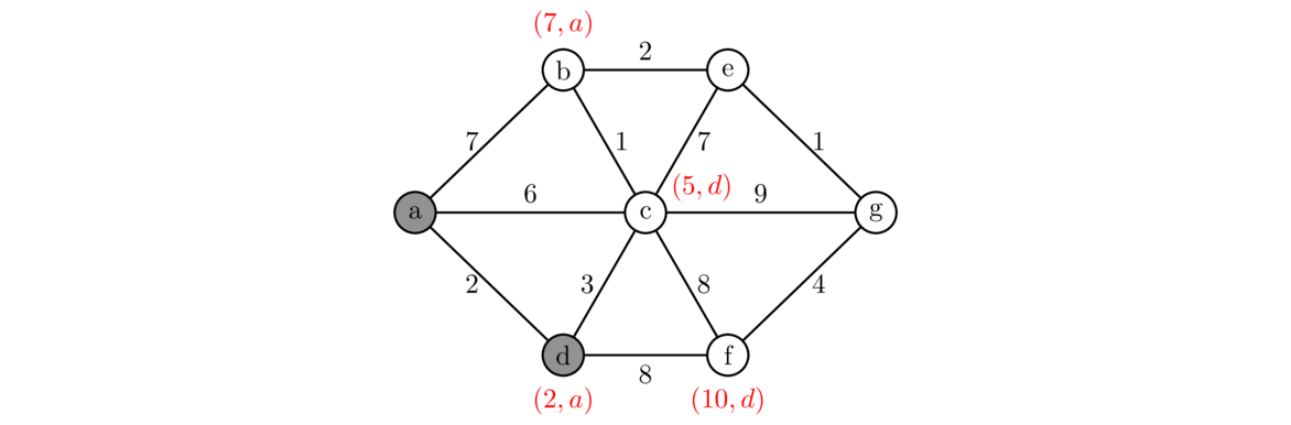
Use Dijkstra's algorithm to find a minimum weight path from a to g in the graph below. Please indicate the labels on the vertices in the way we did in these notes and also indicate the order in which the vertices are processed.
The table below gives the cost of building a road between various cities. An entry of ∞ indicates that the road cannot be built. Find the minimum cost of a network of roads such that it is possible to get from any city to any other.

a b c d e
a 0 3 5 11 9
b 3 0 3 9 8
c 5 3 0 ∞ 10
d 11 9 ∞ 0 7
e 9 8 10 7 10
In a weighted graph, people are often interested in the cheapest path between two vertices u and v. One possible approach could be to find a minimum spanning tree and use the path in it between u and v as the cheapest path. Give an example to show why this approach will not always work.
We proved that a tree with n vertices has n-1 edges. Give an example of a simple graph with 5 vertices and 4 edges that isn't a tree.
1. What does it mean to say a graph is 0-regular? What must such graphs look like?
2. Are there any 0-regular trees? Explain.
3. What can you say about 1-regular trees? Explain.
4. Explain why there cannot exist a k-regular tree if k ≥ 2.
Explain why Dijkstra's algorithm can stop when the current vertex being processed is the goal vertex, even if there are other vertices in the graph that haven't yet been processed.
Suppose that you are given a Python function called min_span(G) that is given a weighted graph G and returns a minimum spanning tree of that graph. The code for that function uses some crazy Python tricks and you don't want to mess with it at all. Suppose you now have a graph G and need to find a maximum spanning tree (spanning tree with the largest possible total weight). Explain how you can use the min_span(G) function to find the maximum spanning tree simply by altering the input graph G in a particular way.
Suppose you are given a program that uses Dijkstra's algorithm on weighted graphs. Describe how to use that program (without modifying it) to find the shortest path between two vertices in an unweighted graph.
Prim's and Kruskal's algorithms work fine with negative weights, but Dijkstra's algorithm doesn't. Give an example to show that Dijkstra's algorithm can get caught in an infinite loop with a negative weight, if we allow the algorithm to revisit vertices it has already searched.
One problem in routing packets on a network is that packets can get caught in infinite loops. A solution to that problem is to find a reduced version of the network that has no loops, yet where it is still possible to get from any vertex to any other. How do you solve this problem with graph theory?
Suppose we have found a MST of a graph. A little later we find we need to add a vertex v to the graph, along with edges from it to some of the other vertices in the graph. A colleague suggests that rather than rerun the MST algorithm, we could just add the cheapest edge from v, and this would give us a MST of the new graph. Show via a small example that this approach won't always work.
Show why the following minimum spanning tree algorithm will not work: Start at any vertex and always add the minimum weight edge from the most recently added vertex.
Our MST algorithms find the spanning tree where the sum of the edge weights is as small as possible. We can use these algorithms also to find a spanning tree where the product of the edge weights is as small as possible. The trick is to replace each edge weight with its logarithm and then run the MST algorithm on that graph. Explain why this works.
If a graph is disconnected, Kruskal's algorithm will not return a MST, but it will return something useful. What will it return?
Which trees on n vertices have
1. Prüfer codes that consist of only one value (e.g. (3,3,3,…,3))?
2. Prüfer codes that consist of exactly two values? (e.g. (3,2,2,3,3,2,2,…))?
3. Prüfer codes that have distinct values in all positions?
Find a formula for the number of spanning trees of the complete bipartite graph K_2,n. You can do this either by starting with K_2,1 and K_2,2 and building up from there using the τ(G) = τ(G-e)+τ(G · e) formula, or you can do it with the Matrix tree theorem if you know how to compute determinants.
Prove that K_n is bipartite if and only if n ≤ 2.
Suppose G and H are both bipartite graphs. Prove that G ∪ H is bipartite.
Prove that if G and H are graphs where G contains at least one edge and H contains at least one vertex, then G∨ H cannot be bipartite.
Prove that if G is a bipartite graph with at least 5 vertices, then G cannot be bipartite.
Prove that if G is bipartite and k-regular, then both partite sets must have the same size.
Prove that if G and H are both bipartite, then G □ H is also bipartite.
Prove that a k-regular graph where k ≥ 2 cannot be a tree.
Prove that in every forest with n vertices, e edges, and c components, we must have n-e = c.
Prove that every tree that has a vertex of degree k has at least k leaves.
Prove that if all the edges of a graph have different weights, then there is a unique minimum spanning tree of that graph.
Write a function distance(G, u, v) that returns the distance in the graph G from u to v. The distance is the length of the shortest path (in terms of number of edges) between the two vertices.
Write a function called adjacency_matrix(G) that takes a graph G as its parameter and returns the adjacency matrix of G as a two-dimensional list/array.
Create a function is_bipartite(G) that determines if a graph is bipartite.
Write a function called prufer_encode(T) that takes a labeled tree T as a parameter and returns the Prüfer code of that graph. In Python, a labeled tree can simply be a tree with integer vertices.
Write a function called prufer_decode(S) that takes a sequence of integers S as a parameter and returns the labeled tree from Prüfer decoding.
Write a function called contract(G, e) that takes a graph G and an edge e of G and returns G · e, the graph obtained by contracting edge e.
Write a function called tau(G) that uses the τ(G) = τ(G-e)+τ(G · e) formula to compute the number of spanning trees of G.
Write a function called tau2(G) that takes a graph and returns the number of spanning trees it has by using the Matrix tree theorem. To get the determinant in Python, you will want to download and import numpy (which is very useful) and use numpy.linalg.det().

Exercises for Chapter 4

Using the graphs below, find an Eulerian circuit and a cycle decomposition. Please indicate the order in which you visit the edges for the circuit, and please indicate your cycle decomposition clearly.
Find Hamiltonian cycles in the graphs below.
Use the vertex deletion criterion to show the graphs below have no Hamiltonian cycle.
Suppose we have a simple graph G that has k odd vertices. Describe a process to create an Eulerian simple graph H that has G as a subgraph. Your process should do this by adding some vertices and edges to the graph, and it should add no more than k/2 new vertices to the graph. Make sure your process works in general and not just for a single example.
The degrees of the 10 vertices in a simple graph are 4,4,7,7,7,7,8,8,8,8.
1. Is this graph Eulerian? Explain.
2. Is this graph Hamiltonian? Explain.
Find the closure of the graph below.
Below are the sequences of degrees in from several graphs. Which of Dirac's, Pósa's, and Chvátal's conditions are satisfied? Give a brief explanation for each. [Note: there are nine separate things to answer for this question.]
1. 6 7 7 7 7 7 7 7 7 8
2. 2 3 4 6 6 6 6 6 6 9
3. 2 2 4 5 6 6 7 8 9 9
Give an example of a graph with exactly five vertices for which Dirac's condition is not satisfied but Ore's condition is. Explain briefly.
Consider the following conditions for Hamiltonian cycles: Dirac's condition, Ore's condition, the Bondy-Chvátal condition, Pósa's condition, and Chvátal's condition. Which conditions can be used to show the graph below has a Hamiltonian cycle and which can't? Give a short explanation for each.
True or False. No reasons needed.
1. Most mathematicians expect that a polynomial-time algorithm for Hamiltonian cycles will be found within the next few decades.
2. No one has yet found a polynomial-time algorithm to find Eulerian circuits.
3. Suppose G fails Chvátal's condition. Then G does not have a Hamiltonian cycle.
4. Suppose G fails the Euler circuit criterion. Then G doesn't have an Eulerian circuit.
5. Suppose the deletion of two vertices breaks G into three components. Then G has no Hamiltonian cycle.
6. Suppose for every set S, G-S has no more than |S| components. Then G has a Hamiltonian cycle.
7. If the closure of G turns out to be K_n,n, where n ≥ 2, then G is Hamiltonian.
8. It is possible for a tree to contain a Hamiltonian cycle.
9. Any connected graph with 10 vertices and 15 edges must contain a cycle.
10. Dirac's condition is usually used to show that a graph is not Hamiltonian.
11. For n ≥ 2, Dirac's condition can be used show K_n,n is Hamiltonian.
Explain why the following problem is NP:

Given a graph with N vertices, determine if there is a collection of no more than k vertices such that every edge in the graph is incident on one of those vertices.
Suppose I give you a program that finds the optimal solution to the Traveling salesman problem. The program takes a weighted complete graph and returns a minimum weight Hamiltonian cycle of that graph. Describe how you can use my program, without changing any of its code, to find a Hamiltonian cycle in an unweighted Hamiltonian graph G that is also not necessarily a complete graph. Do this by describing how to alter G into something you can feed into the program and then describing how to use the program's output to find a Hamiltonian cycle in G.
Show that the complete bipartite graph K_n,n has ^{(n-1)! m!}/₂ Hamiltonian cycles.
Give a single condition that is both necessary and sufficient for a graph to be decomposable into a collection C of subgraphs, where every subgraph in C is a cycle except for one, which is a path.
Prove that the criterion you gave in problem 14 is correct.
A Hamiltonian path is a path in a graph that includes every vertex. Prove that a graph G has a Hamiltonian path if and only if G∨ K₁ has a Hamiltonian cycle.
For each of the following, either give a logical proof of its correctness, or give a counterexample to show it is false.
1. Suppose G and H are both Eulerian. Prove or disprove that G∨ H is Eulerian.
2. Suppose G and H are both Hamiltonian. Prove or disprove that G∨ H is Hamiltonian.
Suppose G is a connected k-regular simple graph and that G is also connected. Prove that either G or G must be Eulerian.
Prove that C_n is Hamiltonian, if n>4.
Prove that any bipartite graph whose partite sets differ in size by more than 1 vertex is not Hamiltonian.
Suppose G and H are both Eulerian. Prove that G □ H is Eulerian.
Suppose G and H are both Hamiltonian. Prove that G □ H is Hamiltonian.
Write a function called is_eulerian(G) that returns whether or not a graph G is Eulerian.

Exercises for Chapter 5

Properly color the graphs below using as few colors as possible.
Properly color the graphs below using as few colors as possible.
Edge-color the following graphs using the least amount of colors.
Use the procedure described in Section 5.1 to color the Cartesian product of the graphs below. Be sure to show clearly how the procedure is used. It is not enough to only show the final coloring.
Use the graph below for this problem.
1. Color its edges using the minimum number of colors.
2. We have three inequalities that give us information about the chromatic number. What does each of them have to say about the chromatic number of this graph?
Use the greedy algorithm to find a proper coloring of the graph below on the left. Be sure to specify the ordering you choose.
Fill in the entries inside the vertices in the graph above on the right with an ordering that causes greedy coloring to end up using 3 colors.
Apply Mycielski's construction to K_1,3 and sketch the resulting graph.

Several students are going on a trip together. Problem is, they don't all get along, so some of them can't travel together in the same car. Below is a table of which students get along and which don't. An X indicates that the two students don't get along and an empty slot indicates they do get along. Use graph coloring to determine the minimum number of cars the students will need, assuming students that don't get along must be in different cars. Please indicate which car each student should ride in.

	A	B	C	D	E	F	G	H
A		X			X	X
B	X		X		X		X
C		X		X			X
D			X			X	X	X
E	X	X				X	X	X
F	X			X	X			X
G		X	X	X	X			X
H				X	X	X	X

There are a total of 7 people taking exams. There are 9 different choices of subjects for the exams, and each person has to choose 3 of them. The exams are given Monday, Wednesday, and Friday at 9am. Each subject's exam can only be given at one of those times.
The are Analysis, Algebra, Topology, Discrete Structures, Probability, Statistics, Geometry, Differential Equations, and Functional Analysis. We will abbreviate these with the letters A through I. Below is a list of the exams each student will be taking. Use graph coloring to determine if it possible to schedule the exams so no student would be scheduled for two exams at once. Your answer should either tell which exams should be given on which days or explain why it would not be possible.
1 (A,C,D) 2 (A,E,F) 3 (A,E,I) 4 (B,C,D) 5 (B,D,H) 6 (B,D,H) 7 (B,C,G)
A badminton tournament is planned with students from several schools. The students are A, B, and C from school #1, D and E from school #2, and F and G from school #3. Everyone is supposed to play everyone else in the tournament except that players from the same school are not supposed to play each other. Also, no player should play two matches in the same day. What is the minimum number of days needed to schedule the tournament? Represent this tournament with a graph and use edge coloring to solve the problem.
True or false.
1. For any graphs G and H, χ(G ∪ H) = χ(G) + χ(H).
2. There exists a graph with no triangles and chromatic number 10.
3. If G doesn't contain any cliques of size 3 or greater, then χ(G) ≤ 2.
4. If G is a tripartite graph (all the vertices fit into three sets X, Y, or Z with no edges within a set), then χ(G) ≤ 3.
5. Mycielski's construction shows that it is possible to have triangle-free graphs with a very large chromatic number.
The degrees of the 10 vertices in a simple graph are 4,4,7,7,7,7,8,8,8,8.
1. What is the largest possible value of χ(G), according to a theorem?
2. What are the possible values of χ'(G), according to a theorem?
Suppose we have graphs G₁, G₂, and G₃. Consider the graph H obtained by joining every vertex of G₁ to every vertex of both G₂ and G₃ (but G₂ is not joined to G₃ in this way). Give a formula for χ(H) in terms of χ(G₁), χ(G₂), and χ(G₃), and prove that your formula is correct.
A proper coloring of the rightmost graph of Problem 2 requires four colors. Prove that it cannot be colored with three colors or less.
Just using the inequalities given in the chapter, without actually coloring anything, prove that the graph from problem 6 has chromatic number 4.
Suppose a graph G has one independent set of size 5. All other independent sets in the graph have size 4 or less. Suppose also that the graph has exactly 45 vertices. According to Theorem 21, χ(G) ≥ 9, but if you adapt the ideas in the theorem's proof, it is possible to show that χ(G) ≥ 11. Show how this works.
For any connected graph that is not complete and not an odd cycle, prove that α ≥ n/Δ, where α is the maximum size of an independent set, n is the number of vertices, and Δ is the largest vertex degree. Do this by combining theorems.
Prove that for any graph G there exists an ordering such that greedy coloring with that ordering will use exactly χ(G) colors.
Write a Python function implementing the greedy coloring algorithm. Your function can pick whatever ordering it wants.

Exercises for Chapter 6

Redraw the graphs below with no crossings (hence showing they are planar).
True or false.
1. All trees are planar.
2. A planar graph cannot contain vertices of degree greater than 5.
1. A simple graph with 10 vertices has 30 edges. Is it planar or not or can't we tell?
2. A simple graph with 10 vertices has 20 edges. Is it planar or not or can't we tell?
3. A simple graph with 10 vertices has 2 edges. Is it planar or not or can't we tell?
Euler's formula states that v-e+f = 2. If the graph is 3-regular planar graph, it is possible to rewrite Euler's formula so that it depends on only v and f (and not on e). Do so.
In our development of the fact that there are only five Platonic solids, we had j representing the degree of each vertex, and k representing the number of edges around each face. In particular, j = 5, k = 3 corresponds to the icosahedron. Explain why that is.
Find a subdivision of K_3,3 or K₅ in the graphs below (hence showing the graphs are not planar). Please be clear as to which vertices are used to subdivide edges.
1. Find a subdivision of K_3,3 or K₅ in the graphs below (hence showing the graphs are not planar). Please be clear as to which vertices are used to subdivide edges.
2. Find embeddings of the graphs below on the torus. Please draw your embedding on the rectangular version of the torus.
3. Can any of the graphs below be embedded on a sphere? Explain.
4. Can any of the graphs below be embedded in 3-space? Explain.
Give an example of a 5-regular planar graph.
Euler's formula is only true for connected graphs. But more generally, the following holds: v+e-f = c+1, where c is the number of components in the graph. Explain why this is true.
The vertices of a simple graph have degrees 3,4,4,5,6,6. Prove that the graph is not planar.
The degrees of the 10 vertices in a simple graph are 4,4,7,7,7,7,8,8,8,8. Prove that the graph is not planar.
Prove or disprove: Any graph with at least 1024 edges cannot be planar.
Prove that no k-regular graph can be planar when k ≥ 6.
Euler's formula can be proved via induction on the number of vertices. The key idea used in the induction step is to pick any edge and contract it (pinching operation we learned about earlier). Provide all the details in a correct induction proof.
Prove that no 4-regular bipartite graph can be planar.
Prove that C_n is not planar when n ≥ 8.
Prove that a planar graph with v ≤ 11 vertices must have a vertex of degree at most 4.

Exercises for Chapter 7

Compute α, α', β, and β' for the graphs below. For each, give an example of an appropriate set of vertices or edges that gives the maximum or minimum.
Give an example of a connected graph G with 10 vertices and α(G) = 8.
For each of α, α', β, β', characterize the simple graphs for which the value of the parameter is 1. (i.e., find descriptions of all possible graphs that have α = 1, all possible graphs with α' = 1, etc.)
True/False: In any graph with no isolated vertices, we must have α+β = α'+β'.
A graph has a cover of size 5. What can you say about the size of the largest matching in the graph? Circle all that apply.
(a) It is of size exactly 5.
(b) It is of size exactly 5 if the graph is bipartite.
(c) It is 5 or larger.
(d) It is 5 or smaller.
Suppose G is a graph for which we have found a matching of size 6 as well as a vertex cover of size 6. List all the possible values for α' and β, being as specific as possible (i.e., saying α',β ∈ ℝ would be true but not a good answer).
Given a matching of size m in a graph, describe a process that converts that matching into an edge cover of size at most n-2m, where n is the number of vertices in the graph.
Consider an edge cover in a graph. If we look at the subgraph consisting only of the edges in the cover and their endpoints, each component of that graph must be what type of graph?
A matching is shown in the graph below on the left. Use the augmenting path algorithm to find a larger matching. Please indicate what the augmenting path is and how it is used to create a larger matching.
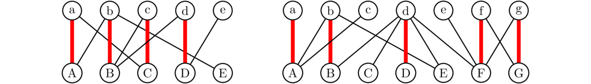
In the graph above on the right a maximum matching is shown. Prove that it is the maximum matching using the process given in the chapter to find the sets S and T such that (X-S) ∪ T is a minimum vertex cover.
A matching is shown in the graph below on the left. Use the augmenting path algorithm to find a larger matching. Please indicate what the augmenting path is and how it is used to create a larger matching.
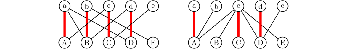
In the graph above on the right a maximum matching is shown. Prove that it is the maximum matching using the process given in the chapter to find the sets S and T such that (X-S) ∪ T is a minimum vertex cover.
Use Hall's theorem to explain why the graph above on the right does not have a perfect matching.
Use Hall's theorem to explain why the graph below does not have a perfect matching.
Alice, Bob, Chris, Dave, Ed, and Fred are math students trying to sign up for courses that are nearly full. There are seven courses that are still open, and each only has one seat left. The courses are 1. Calculus, 2. Algebra, 3. Geometry, 4. Topology, 5. Probability, 6. Statistics, and 7. Eighteenth Century British Literature. This list below gives the classes each student would be happy taking. Is is possible for everyone to get a course they like? Do this problem by setting up a bipartite graph and looking for a maximum matching.
```
     A: 1,3    B: 2    C: 1,5    D:3,4,5    E: 2,6    F:5,7
```
Suppose we want to place ATMs around a city so that no one ever has to walk more than 1 block to get to an ATM. Describe how to use one of the following in order to solve the ATM problem as efficiently as possible: independent set of vertices, independent set of edges, vertex cover, edge cover.
Use the Hungarian algorithm to find an optimal assignment in the matrices given below.

a b c d
A 3 3 7 1
B 9 7 5 2
C 7 6 2 4
D 9 9 4 7

a b c d
A 2 6 8 9
B 5 3 4 6
C 1 4 8 7
D 3 2 6 7
Suppose the men are named a, b, c, and d, and the women are named w, x, y, z. Preference lists are below for two separate problems. Use the Gale-Shapely algorithm to find a stable matching for each. Please indicate each step in a table like we did in the chapter.

a: xzwy w: abcd a: wxyz w: cbad

b: zwyx x: abdc b: xywz x: acbd

c: wzxy y: cbad c: zyxw y: cadb

d: zwyx z: dacb d: xwzy z: dcba

Exercises for Chapter 8

In a digraph, we can list the degrees of the vertices with an ordered pair, like (d^-,d⁺), where d^- is the indegree and d⁺ is the outdegree. Can there exist a digraph on 4 vertices whose degrees are (2,1), (2,1), (1,2), and (2,2)? Explain.
Find an orientation of the Petersen graph that has no directed cycles.
Explain why the digraph below on the left is weakly connected, but not strongly connected.
Is the digraph in the middle above weakly connected, strongly connected, or neither?
Find the strong components in the digraph on the right above.
Topologically sort the DAGs below.
Find the error in the following algorithm to topologically sort a connected DAG: Looping over all vertices of indegree 0, run a BFS from each vertex. Label the vertices in the order that BFS finds them. That ordering is a topological order.
Suppose we have 20 different jobs to be done. Some of those jobs can't be done until others are done. We want to find a way to order the jobs so that no job is scheduled to be done before another job that is a prerequisite for that job. Describe how to use graph theory to order the jobs.
Describe an algorithm that determines if a DAG contains a vertex that is reachable from all other vertices. [Hint: Use the topological sort and then work your way from the back to the front.]
Finding a Hamiltonian path in a general digraph is hard, but in a DAG it is easy. Describe how to use a topological sort to find a Hamiltonian path in a DAG.
A DAG can have multiple topological orders. Prove that a DAG has a unique topological ordering if and only if it has a Hamiltonian path.
In a DAG, there is a faster way to find a minimum weight path than using Dijkstra's algorithm. Implement the following algorithm: Topologically sort the vertices. Then process the vertices in that order, maintaining for each vertex the current best cost to it from vertices before it in the order.

Exercises for Chapter 9

Find κ and κ' for the graphs below.
What are the blocks of the graph above on the left?
Show that Menger's theorem works for the graphs below by finding a set of k vertices that separates x from y and finding k paths from x to y that share no vertices besides x and y.
Shown below are flows on digraphs. The labels on the edges are in the form x|y, where x is the flow amount and y is the capacity. Assume the source is a and the sink is h.
1. Use the Ford-Fulkerson algorithm to find a maximum flow on that digraph, starting with the given flow. It should take two steps. Please indicate clearly how both of those steps work.
2. Use the Ford-Fulkerson algorithm to find a minimum cut of the same size as the maximum flow.
A graph has a cut edge. What are the possible values of κ and κ'?
Give an example of a simple graph or multigraph with κ = 2 and κ' = 5.
Give an example of a simple graph or multigraph with κ = 1 and κ' = 5. Describe how to generalize your example to create a graph with κ = 1 and κ' arbitrarily large.
The augmenting path algorithm and the Ford-Fulkerson algorithm are examples of a technique known as iterative improvement. Explain what about these algorithms makes that name appropriate.
The Ford-Fulkerson algorithm looks for paths from the source where all the forward edges along the path are under capacity and all the backwards edges have positive flow. When it finds such a path, it augments the flow by adding 1 to the flow on the forward edges and decreasing the flow by 1 on the backward edges. Explain the part about the backward edges, using an example. How does doing this lead to a better flow?
Explain how to use the Ford-Fulkerson algorithm to handle a network flow problem where there are multiple sources and multiple sinks. [Hint: Create a new graph with a single source and sink such that a maximum flow in the new graph would solve the original multiple source/sink problem.]
Explain how to use network flow to determine how many edge-disjoint paths there are in a directed graph between two given vertices. [Edge-disjoint means the paths don't have any edges in common.]
Prove that if G is a graph that consists of blocks B₁ and B₂, then χ(G) = max(χ(B₁), χ(B₂)).

a:	xzwy	w:	abcd	a:	wxyz	w:	cbad
b:	zwyx	x:	abdc	b:	xywz	x:	acbd
c:	wzxy	y:	cbad	c:	zyxw	y:	cadb
d:	zwyx	z:	dacb	d:	xwzy	z:	dcba

	a	b	c	d	e
a	0	3	5	11	9
b	3	0	3	9	8
c	5	3	0	∞	10
d	11	9	∞	0	7
e	9	8	10	7	10