Notes for Number Theory
© 2019 Brian Heinold Here is a pdf version of the book.
Here are the notes I wrote up for a number theory course I taught. The notes cover elementary number theory but don't get into anything too advanced. My approach to things is fairly informal. I like to explain the ideas behind everything without getting too formal and also without getting too wordy.
If you see anything wrong (including typos), please send me a note at heinold@msmary.edu.
One of the most basic concepts in number theory is that of divisibility. The concept is familiar: 14 is divisible by 7, even numbers are divisible by 2, prime numbers are only divisible by themselves and 1, etc. Here is the formal definition:
For example, 20 is divisible by 4 because we can write 20 = 4 · 5; that is n = dk, with n = 20, d = 4, and k = 5. The equation n = dk is the key part of the definition. It gives us a formula that we can associate with the concept of divisibility.
This formula is handy when it comes to proving things involving divisibility. If we are given that n is divisible by d, then we write that in equation form as n = dk for some integer k. If we need to show that n is divisible by d, then we need to find some integer k such that n = dk.
Here are a few example proofs:
Proof. Even numbers are divisible by 2, so we can write n = 2k for some integer k. Then n2 = (2k)2 = 4k2, which we can write as n2 = 2(2k2). We have written n2 as 2 times some integer, so we see that n2 is divisible by 2 (and hence even).◻
Proof. Since a ∣ b and b ∣ c we can write b = aj and c = bk for some integers j and k.**Note that we must use different integers here since the integer j that works for a ∣ b does not necessarily equal the integer k that works for b ∣ c. Plug the first equation into the second to get c = (aj)k, which we can rewrite as c = a(jk). So we see that a ∣ c, since we have written c as a multiple of a. ◻
Proof. Since a ∣ b, we can write b = ak for some integer k. Multiply both sides of this equation by c to get (ac)k = bc. This equation tells us that ac ∣ bc, which is what we want.◻
Here are a couple of other divisibility examples:
Solution. All we need is a single counterexample. Setting a = 5, b = 3, and c = 7 does the trick.
Solution. The only answers are 593 and 607. It would be tedious to find them by checking divisors starting with 2, 3, etc. A better way is to use the algebraic fact x2–y2 = (x–y)(x+y). This fact is very useful in number theory.
With a little cleverness, we might notice that 359951 is 360000–49, which is 6002–72. We can factor this into (600–7)(600+7), or 593 × 607.
The division algorithm, despite its name, it is not really an algorithm. It states that when you divide two numbers, there is a unique quotient and remainder. Specifically, it says the following:
The integers q and r are called the quotient and remainder. For example, if a = 27 and b = 7, then q = 3 and r = 6. That is, 27 ÷7 is 3 with a remainder of 6, or in equation form: 27 = 7 · 3+6. The proof of the theorem is not difficult and can be found in number theory textbooks.
One of the keys here is that the remainder is less than b. Here are some consequences of the theorem:
We see that in each case, n3–n is divisible by 3. By the division algorithm, these are the only cases we need to check, since every integer must be of one of those three forms.
Proof. Every integer n is of the form 2k or 2k+1.
If n = 2k, then we have n2 = 4k2, which is of the form 4k.**We are being a bit informal here with the notation. When we say the number is of the form 4k, the k is different from the k used in n = 2k. What we're really saying here is that the number is of the form 4 times some integer. A more rigorous way to approach this might be to let n = 2j, compute n2 = 4j2 and say n2 = 4k, with k = j2.
If n = 2j+1, then we have n2 = 4k2+4k+1 = 4(k2+k) + 1, which is of the form 4k+1.
◻
Proof. Every integer is of the form 6k, 6k+1, 6k+2, 6k+3, 6k+4, or 6k+5. An integer of form 6k is divisible by 6. A integer of the form 6k+2 is divisible by 2 as it can be written as 2(3k+1). Similarly, an integer of the form 6k+3 is divisible by 3 and an integer of the form 6k+4 is divisible by 2. None of these forms can be prime (except for the integers 2 and 3, which we exclude), so the only forms left that could be prime are 6k+1 and 6k+5.◻
Proof. We will start by writing a4+b4–2 as (a4–1) + (b4–1). Let's take a look at the a4–1 term. We can factor that into (a2–1)(a2+1) and further into (a–1)(a+1)(a2+1). Since we know a is odd, we can write a = 2k+1 and we have
So we have that a4–1 is divisible by 16. A similar argument tells us that b4–1 is divisible by 16, and from there we get that a4+b4–2 is divisible by 16, since it is the sum of two multiples of 16.
◻
Proof. First, note that the square of an even is even and the square of an odd is odd since (2k)2 = 2(2k2) is even and (2k+1)2 = 2(2k2+2k)+1 is odd. In particular, if an integer a2 is even, then a is even as well.
Suppose √2 = p/q, with p and q positive integers. By clearing common factors, we can assume the fraction is in lowest terms. Multiply both sides by q and square both sides to get 2q2 = p2. This tells us that 2 ∣ p2. Thus 2 ∣ p by the statement above, and we can write p = 2k for some integer k. So we have 2q2 = (2k)2, which simplifies to q2 = 2k2. This tells us that 2 ∣ q2 and hence 2 ∣ q. But this is a problem because p and q both have a factor of 2 and p/q is supposed to already be in lowest terms. So we have a contradiction, which shows that it must not be possible to write √2 as a ratio of integers.
It is not to hard to extend this result to show that n√m is irrational unless m is a perfect nth power.
The second example above is sometimes useful when working with perfect squares. We record it as a theorem:
For example, 3999 is not a perfect square since it is 4000–1, which is of the form 4k–1 (same as a 4k+3 form). On the other hand, just because something is of the form 4k+1 does not mean it is a perfect square. For instance, 41 is of the form 4k+1, but isn't a perfect square.
As another example, 3n2–1 is not a perfect square for any integer n. To see this, break the problem into two cases: n = 2k and n = 2k+1. If n = 2k, then 3n2–1 = 3(4k2)–1 = 4(3k2)–1. If n = 2k+1, then 3n2–1 = 3(4k2+4k+1)–1 = 4(3k2+3k)+2. Neither of these are of the form 4k or 4k+1, so they are not perfect squares.
Similar results to the theorem above can be proved for other integers. For instance, every perfect square is of the form 5k, 5k+1, or 5k+4.
Note that we can also take the remainders to be in other ranges besides from 0 to b–1. The most useful range is from –b/2 and b/2. For instance, with b = 3, we can also write every integer as being of the form 3k–1, 3k, or 3k+1. An integer of the form 3k–1 is also of the form 3k+2. As another example, we can write every integer in one of the forms 6k–2, 6k–1, 6k, 6k+1, 6k+2, or 6k+3.
In grammar school, the remainder always seemed to me to be an afterthought, but in higher math, it is quite useful and important. It is built into most programming languages, usually with the symbol mod or %
For example, suppose we want to find 68 mod 7. The definition above tells us to find the nearest multiple of 7 less than n and subtract. The closest multiple of 7 less than 68 is 63, and 68–63 = 5. So 68 mod 7 = 5.
This procedure applies to negatives as well. For instance, to compute –31 mod 5, the closest multiple of 5 less than or equal to -31 is -35, which is 4 away from -31, so –31 mod 5 = 4, or –31 ≡ 4 (mod 5).
As one further example, suppose we want 179 mod 18. 179 is one less than 180, a multiple of 18, so it leaves a remainder of 18-1 = 17. So 179 mod 18 = 17.
A nice way to compute mods mentally or by hand is to use a streamlined version of the grade school long division algorithm. For example, suppose we want to compute 34529 mod 7. Here is the procedure:
The end result is 34529 mod 7 = 5.
For example, the gcd of 24 and 96 is 12, since 12 is the largest integer that divides both 24 and 96. As another example, the gcd of 18 and 25 is 1. Those numbers have no divisors in common besides 1.
To find the gcd of two integers, the Euclidean algorithm is used. We'll start with an example, finding gcd(21, 78):
In general, to find gcd(a, b), assume a ≤ b, and compute
The reason it works is that the common divisors of a and b are exactly the same as the common divisors as a and b mod a, so their gcds must be the same. Because of this, when we apply the Euclidean algorithm, the gcd of the two numbers on the left side stays constant all the way through the algorithm. For example, when we compute gcd(21, 78), we get the following:
It is worth showing why the common divisors of a and b are the same as the common divisors as a and b mod a. First, when we apply the division algorithm to a and b, we get b = aq + r, where r = b mod a. If a and b are both divisible by some common divisor d, then r = b–aq will be as well, since we can factor d out of the right side. On the other hand, if a and r are both divisible by some common divisor d, then b = r–aq will be as well, since we can factor d out of the right side.
In number theory, a linear combination of the integers a and b is an expression of the form ax+by for some integers x and y. For example, a linear combination of a = 6 and b = 15 is an expression of the form 6x+15y, like 6(1)+15(2) = 36 or 6(4)+15(–1) = 9. Linear combinations are important in a variety of contexts.
Linear combinations have a close connection with the gcd. Suppose we want to know if it is possible to write 4 as a linear combination of 6 and 15. That is, can we find integers x and y such that 6x+15y = 4? The answer is no, since the left side is a multiple of 3 (namely 3(2x+5y)), but the right side is not a multiple of 3. By the same reasoning, in general, if c is not a multiple of gcd(a, b), then it is impossible to write c as a linear combination of a and b.
What about multiples of the gcd? Is it always possible to write ax+by = c if c is a multiple of the gcd? The answer is yes. We just have to show how to write the gcd as a linear combination of a and b. Once we have this (see the proof below for how), we can then multiply through to get c. For instance, suppose we want to find x and y such that 6x+15y = 21. We have gcd(6, 15) = 3 and it is not hard to find that 6(3)+15(–1) = 3. If we multiply through by 7, we get 6(21)+15(–7) = 21. So it just comes down to writing the gcd as a linear combination.
Here is a formal statement of the above along with a proof:
We now show that it is possible to write d as a linear combination of a and b. Start by letting e be the smallest positive linear combination of a and b. We need to show that e = d.
Finally, if c is a multiple of d (say c = dk for some integer k), and we have integers x and y such that ax+by = d, then we can multiply through by k to get a(kx)+b(ky) = c.
In particular, we have the following important special case:
This fact is useful when working with gcds because it gives us an equation to work with. On the other hand, be careful. Just because we can write ax+by = c, that does not mean c = gcd(a, b). All we are guaranteed is that c is a multiple of gcd(a, b).
Theorem 3 tells us that the gcd is a linear combination, but it doesn't tell us how to find that linear combination. Being able to find that linear combination is important in a number of contexts. The trick is to use the Euclidean algorithm in a particular way.
In the earlier example when we found gcd(21, 78) using the Euclidean algorithm, we used the modulo operation. Written out fully using the division algorithm, the Euclidean algorithm on this example is as follows:
We can use this sequence of steps to find the linear combination by working backwards. Start with the second-to-last equation from the Euclidean algorithm and work back up in the following way:
Note that at each step we can check our work by making sure the expression equals the gcd. For instance, in the third line above, 15(3)–21(2) = 45–42 = 3.
Here is another example. Suppose we want to find integers such that 11x+41y = 1. Start with the Euclidean algorithm:
Thus we have x = 15 and y = –4 that give us 11x+41y = 1.
This algorithm is called the extended Euclidean algorithm. It turns out to have a number of important uses, as we will see.
Here is a short Python program implementing a version of it. This is a streamlined version of the algebra above, based on the algorithm given at http://en.wikipedia.org/wiki/Extended_Euclidean_algorithm.
The keys to many proofs involving gcds are as follows:
Here are a few example proofs involving gcds:
Proof. The basic idea here is intuitively clear: If we divide through by the gcd, then what's left should not have factors in common, since all the common factors should be in the gcd.
Here is a more algebraic approach: Start by writing ax+by = d for some integers x and y. We can then divide through by d to get (a/d)x + (b/d)y = 1. Theorem 3 tell us that gcd(a/d, b/d) divides any linear combination of a/d and b/d. So gcd(a/d, b/d) is a divisor of 1, meaning it must equal 1.◻
Proof. Write c = aj, c = bk, and d = ax+by for some integers j, k, x, and y. Multiply the last equation through by c to get cd = acx+bcy. Then plug in c = bk into the acx term and c = aj into the bcy term to get cd = abkx + bajy. So we have cd = ab(kx+jy), showing that ab ∣ cd.◻
Proof. Let d = gcd(a, b) and d′ = gcd(ka, kb). We can write d = ax+by for some integers x and y. Multiplying through by k gives kd = kax+kby. This is a linear combination of ka and kb, so we know that d′ ∣ kd. On the other hand, we can write d′ = kax′+kby′ for some integers x′ and y′. Divide through by k to get d′/k = ax′+by′. This is a linear combination of a and b, so d ∣ d′/k, or kd ∣ d′. Since d′ ∣ kd and kd ∣ d′, and k > 0, we must have d′ = kd.◻
Proof. Let d1 = gcd(a, c) and d2 = gcd(b, c). From these, we can write ax1+cy1 = d1 and bx2+cy2 = d2 for some integers x1, x2, y1, and y2. Also, since c ∣ (a–b) we can write a–b = ck for some integer k, which we can solve to get a = ck+b and b = a–ck. Plugging the former into the equation for d1 gives (ck+b)x1+cy1 = d1, which we can write as c(kx1+y1)+bx1 = d1. The left hand side is a linear combination of b and c, so it is a multiple of d2 = gcd(b, c). Thus d2 ∣ d1. Plugging b = a–ck into the equation for d2 and doing a similar computation gives d1 ∣ d2. Thus d1 = d2.
◻
A relative of the gcd is the least common multiple.
The following gives an easy way to find the lcm:
Here an example: If a = 14 and b = 16, then gcd(a, b) = 2, ab = 224 and lcm(a, b) = 224/2 = 112. A simple way to think of this theorem is that ab is a multiple of both a and b, but it has some redundant factors in it. Dividing out by gcd(a, b) removes all of the redundancies, leaving the smallest possible common multiple. Here is a formal proof of the theorem:
First, since d is divisor of a and b, we can write a = dk and b = dj. Then ab/d = aj and ab/d = bk, which shows that ab/d is a multiple of both a and b.
Next, let m be any common multiple of a and b. So we have m = as and m = bt for some integers r and s, and we can write 1/a = s/m and 1/b = t/m.
We can also write d as a linear combination d = ax+by for some integers x and y. Dividing both sides of this equation by ab, we get dab = xb + ya. Plugging in our earlier equations for 1/a and 1/b gives dab = xtm + ysm, which we can rewrite as m = (xt+ys)abd. This tells us that ad/b is a divisor of m.
Since m is an arbitrary multiple of a and b, and ab/d divides it, that means that ab/d is the smallest possible multiple, which is what we wanted to prove.
There are other ways to find lcm(a, b). One way would be to list all the multiples of a and all the multiples of b and find the first one they have in common. This, however, is slow unless a and b are small. Another way uses the prime factorization. See Section 2.1 for an example.
Here is a simple example where the lcm is useful. Suppose one thing happens every 28 days and other happens every 30 days, and that both things happened today. When will they both happen again? The answer is lcm(28, 30) = 420 days from now.**A more general approach to handling these kinds of cyclical problems is covered in Section 3.10.
As another example, some people theorize that the timing of periodic cicadas has to do with the lcm. Some species of cicadas only emerge every 13 years, while others emerge every 17 years. People have noticed that these are values are both prime. This means that the lcm of these numbers with other numbers is relatively large. The things that eat cicadas are often on a boom-bust cycle, and it would be bad for cicadas to emerge in a year when there are a lot of predators. Suppose a certain predator is on a 4-year cycle. How often would a boom year coincide with a 13-year cicada emergence? The answer is every lcm(4, 13) = 52 years. On the other hand, if cicadas were on say a 14-year cycle, then it would happen every 28 years. It would also be bad for both the 13-year and the 17-year cicadas to emerge at once, since they would be competing for resources. But this will only happen every lcm(13, 17) = 191 years.
In other words, a and b are relatively prime provided they have no divisors in common besides 1 (or maybe -1 if they are negative). There are a number of facts in number theory that are only true for relatively prime integers. Here is one useful fact that follows quickly from Theorem 3:
One of the most useful tools in number theory is the following result:
For example, if c ∣ (5 × 12), and c has no factors in common with 5, then in order for it to divide 5 × 12 = 60, it must divide 12. On the other hand, if a and c do have factors in common besides 1, then the result might not hold. For instance, if a = 10, then 10 ∣ (5 × 12), but 10 ∤ 12.
The concept of gcd can be applied to more than two integers. Namely, gcd(a1, a2, …, an) is the largest integer that divides each of the ai. For instance, gcd(24, 36, 60) = 12. The gcd can be computed from the Euclidean algorithm and the following fact:
It is also possible to compute the gcd by extending the ideas of the Euclidean algorithm. We perform several modulos at each step, always modding by the smallest value. Here is some (slightly tricky) Python code implementing these ideas:
One thing to be careful of is that it is possible to have gcd(a, b, c) = 1, but not have gcd(a, b) and gcd(b, c) both equal to 1. For instance, gcd(2, 4, 5) = 1 since 1 is the largest integer dividing 2, 4, and 5, but gcd(2, 4)≠ 1.
For many theorems that require a bunch of integers, a1, a2, …, an to not have any factors in common, instead of requiring gcd(a1, a2, …, an) = 1, often the following notion is used:
The lcm of integers a1, a2, …, an is the smallest integer that is a multiple of each of the ai. Similarly to the gcd, the lcm can be computed by using the rule below to break things down.
Here is a list of facts that might come in handy from time to time. It's not worth memorizing this list, but it may be useful to refer back to if you need a certain fact for something you are working on.
Most important facts
Divisibility
Gcds
Prime numbers are one of the main focuses of number theory.
Notice that 1 is not considered to be prime. The reason is that primes are thought of as fundamental building blocks of numbers. As we will soon see, every number is a product of primes, each prime helping to build up the number. However, 1 doesn't do any building, as multiplying by 1 doesn't accomplish anything. There are other ways in which 1 behaves differently from prime numbers, and for these reasons 1 is not considered prime.
The first few primes are 2, 3, 5, 7, 11, 13, 17, 19. Much of number theory is concerned with the structure of the primes—how frequent they are, gaps between them, whether there is any sort of pattern to them, etc.
Recall Euclid's lemma from Section 1.9. It states that if c ∣ ab and gcd(c, a) = 1, then c ∣ b. If a is prime, then gcd(c, a) = 1, so Euclid's lemma holds whenever p is prime. Here is Euclid's lemma restated for primes:
Euclid's lemma could be used as an alternate definition for prime numbers as it is not too hard to show that no other number besides 1 has this property. In fact, Euclid's lemma is used to define analogs of prime numbers (like prime ideals) in abstract algebra.
Using induction, Euclid's lemma can be extended as follows:
A direct consequence of this is the following:
Euclid's lemma is one of the most important tools in elementary number theory and we will see it appear again and again.
In math there are a number of “fundamental theorems.” There is the fundamental theorem of algebra which states that every nonconstant polynomial has a root, the fundamental theorem of calculus that relates integration to differentiation, and in number theory, there is the fundamental theorem of arithmetic, which states that every integer greater than 1 can be factored uniquely into primes. For instance, we can factor 60 into 2 × 2 × 3 × 5 and there is no other product of primes equal to 60, other than changing the order of 2 × 2 × 3 × 5. Here is the formal statement of the theorem:
Here is intuitively why we can write n as a product of primes: Either n itself is prime (in which case we are done) or else n can be factored into a product ab. These integers are either prime or they themselves can be factored. These new factors are in turn either prime or they can be factored. We can continue this process, but eventually it must stop since the factors of a number are smaller than the number itself, and things can't keep getting smaller forever. This can be made formal using induction.
To show the representation is unique, suppose n = p1p2… pk and n = q1q2… qm are two different representations. From the first representation, we have p1 ∣ n, and so p1 ∣ q1q2… qm. By Corollary 10, we must have p1 = qi for some i. By rearranging terms, we can assume i = 1, so p1 = q1. By the same argument, we can similarly conclude that p2 = q2, p3 = q3, etc. Thus the two representations are the same.
In the factorization, some of the primes may be the same, like in 720 = 2 × 2 × 2 × 2 × 3 × 3 × 5. We can gather those factors up and write the factorization as 23 · 32 · 5. In general, we can always write an integer n > 1 as a unique product of the form pe11pe22… pekk.
To get the gcd, we go prime-by-prime through the two representations, always taking the lesser of the two amounts. For instance, both 168 and 180 have a factor of 2: 168 has 23 and 180 has 22, and so we use the lesser factor, 22, in the gcd. Moving on to the factor 3, 168 has 31 and 180 has 32, so we take 31. The next factors are 5 and 7, but they are not common to both 168 and 180, so we ignore them. We end up with gcd(168, 180) = 22 · 3 = 12.
The lcm is done similarly, except that we always take the larger amount. We get lcm(168, 180) = 23 · 32 · 5 · 7 = 2520.
Using the prime factorization to find the gcd and lcm is fast if we have the factorization is available. However, finding the prime factorization is a slow process for large numbers. The Euclidean algorithm is orders of magnitude faster.**A little more formally, the Euclidean algorithm's running time grows linearly with the number of digits in the number, whereas the running times of the fastest known factoring algorithms grow exponentially with the number of digits.
We can write n = m2 for some m and assume m has the prime factorization m = pe11pe22… pekk. Then
Since a ∣ c, every term, peii, in the factorization of a occurs in the factorization of c. Similarly, since b ∣ c, every term in the factorization of b occurs in the factorization of c. Since gcd(a, b) = 1, the primes in the factorization of a must be different from the primes in the factorization of b. Thus every term in the factorization of ab occurs in the factorization of c. So ab ∣ c.
An alternate way to do the above proof would be to assume that there were only finitely many primes and to use the process above to derive a contradiction. A quick web search will turn up dozens of other interesting proofs of the infinitude of primes.
It is worth noting that the integer P in the proof above need not be prime itself. It only needs to be divisible by a new prime. Numbers of the form given in the proof above are sometimes called Euclid numbers or primorials. The first few are
One of the simplest ways to check if a number is prime is trial division. Just check to see if it is divisible by any of the integers 2, 3, 4, etc.
When considering divisors of n, they come in pairs, one less than or equal to √n and the other greater than or equal to √n. For instance, if n = 30, we have √30 ≈ 5.47 and we can write 30 as 2 × 15, 3 × 10, and 5 × 6, with 2, 3, and 5 less than √30 and 6, 10, 15 greater than √30. So, in general, we can stop checking for divisors at √n.
This process can be made more efficient by just checking for divisibility by 2 and by odd numbers, or better yet, checking for divisibility only by primes (provided the number is small or we have a list of primes). For example, to check if 617 is prime, we have √617 = 24.84 and we check to see if it is divisible by 2, 3, 5, 7, 11, 13, 17, 19, and 23. It is not divisible by any of those, so it is prime.
This approach is reasonably fast for small numbers, but for checking the primality of larger numbers, like ones with several hundred digits, there are faster techniques, which we will see later.
To find all the primes less than an integer n, we can use a technique called the sieve of Eratosthenes. Start by listing the integers from 2 to n and cross out all the multiples of 2 after 2. Then cross out all the multiples of 3 after 3. Then cross out all the multiples of 5 after 5. Note that we don't have to cross out the multiples of 4 since they have all already been crossed out as they are multiples of 2. We keep going, crossing out multiples of 7, 11, 13, etc., until we get to √n. At the end, only the primes will be left. Here is what we would get for n = 100:
Here is how we might code it in Python. We create a list of zeroes and ones, with a zero at index i meaning i is not prime and a one meaning i is prime. The list starts off initially with all ones and we gradually cross off all the composites.
The sieve works relatively well for finding small primes. The code above, inefficient though it may be, takes 55 seconds to find all the primes less than 108 on my laptop.
A natural question to ask is how common prime numbers are. An answer to this question and some other questions is given by the prime number theorem, which states that the number of primes less than n is roughly n/ ln n . Formally, we can state it as follows:
The theorem tells us that roughly 100/ ln n percent of the numbers less than n are prime. For n = 1,000,000, the theorem tells us that roughly 7-8% of the numbers less than 1,000,000 are prime, and that around n = 1,000,000 the average gap between primes is roughly ln(1000000) ≈ 14.
The prime number theorem is not easy to prove. The first proofs used sophisticated techniques from complex analysis. There is a proof using only elementary methods, but it is fairly complicated.
The prime number theorem tells us that the probability an integer near x is prime is roughly 1/ ln x. Summing up all these probabilities for all real x from 2 through n gives us another estimate for the number of primes less than n. Such a sum is a continuous sum (an integral), and we get the following estimate for π(n):
An interesting note about this is that for n up through at least 1014 it has been shown that Li(n) < π(n). But it turns out not to be true for all n. In fact, it was proved in 1933 that Li(n)–π(n) changes sign infinitely often. This illustrates an important lesson in number theory: just because something is true for the first trillion (or more) integers, does not mean it is true in general.
The proof is interesting in that it included one of the largest numbers to ever be used in a proof, namely that π(n) < Li(n) for some value less than eee79. More recent research has brought the bound down to e728.
Twin primes are pairs (p, p+2) with both p and p+2 prime. Examples include (5, 7), (11, 13) and (41, 43).
One of the most famous open problems in math is the twin primes conjecture, which asks if there are infinitely many twin primes, Most mathematicians think the conjecture is true, though it is considered to be a very difficult problem.
Referring back to the prime number theorem, we know that the probability an integer near x is prime is roughly 1/ ln x. Assuming independence, the probability that both x and x+2 would be prime is then 1/( ln x)2 and summing up these probabilities gives ∫n2 1( ln x)2 dx as an estimate for the number of twin primes pairs less than n. Independence is not quite a valid assumption here, but it is not too far off. It is currently conjectured that the number of twin prime pairs less than n is approximately 2C2∫n2 1( ln x)2 dx, where C2 ≈ .66016 is something called the twin prime constant.**See Section 1.2 of Prime Numbers: A Computational Perspective, 2nd edition by Crandall and Pomerance for more on this approach.
So it seems reasonable that there are infinitely many twin primes, but it has turned out to be very difficult to prove. The best result so far is that there are infinitely many pairs (p, p+2) where p is prime and p+2 is either prime or the product of two primes, proved by Chen Jingrun in 1973.
There are a number of analogous conjectures. For instance, it is conjectured that there are infinitely many pairs of primes of the form (p, p+4) or infinitely many triples of the form (p, p+2, p+6). Recent work has shown that there are infinitely many primes p such that one of p+2, p+4, … p+246 is also prime.
It is interesting to look at the gaps between consecutive primes. Here are the gaps between the first 100 primes, from 2 to 541:
1, 2, 2, 4, 2, 4, 2, 4, 6, 2, 6, 4, 2, 4, 6, 6, 2, 6, 4, 2, 6, 4, 6, 8, 4, 2, 4, 2, 4, 14, 4, 6, 2, 10, 2, 6, 6, 4, 6, 6, 2, 10, 2, 4, 2, 12, 12, 4, 2, 4, 6, 2, 10, 6, 6, 6, 2, 6, 4, 2, 10, 14, 4, 2, 4, 14, 6, 10, 2, 4, 6, 8, 6, 6, 4, 6, 8, 4, 8, 10, 2, 10, 2, 6, 4, 6, 8, 4, 2, 4, 12, 8, 4, 8, 4, 6, 12, 2, 18
We see gaps of 2 quite often. These correspond to twin primes. There are a few larger gaps, like a gap of 14 from 113 to 127 and a gap of 18 from 523 to 541. It is not too hard to find gaps that are arbitrarily large. Just find an integer n divisible by 2, 3, 4, 5, …, k and then n+2, n+3, … n+k will all be composite.
The prime number theorem tells us that the average gap between a prime p and the next prime is approximately ln p. Thus for p near 1,000,000, we would expect an average gap of about 14, and for p = 10200, we would expect an average gap of around 460.
One important result is relating to prime gaps is Bertrand's postulate.
For example, for n = 1000, we are guaranteed that there is a prime between 1000 and 2000. This is not news, but it is useful in some cases to have an interval on which you are guaranteed to have a prime, even if that interval is rather large.
The proof of Bertrand's postulate is actually not too difficult, but we won't cover it here. There are a number of improvements on Bertrand's postulate. For instance, in 1952 it was proved that for n ≥ 25 there exists a prime between n and (1+15)n. The range can be narrowed further for larger n.**In general, it has been proved that for any ε > 0 there is an integer N such that for n ≥ N, there is always a prime between n and (1+ε)n. In fact, as n → ∞, the number of primes in that range approaches ∞ as well. In math, there are many results concerning how things behave as n approaches ∞. Results of this sort are called asymptotic results.
A related, but unsolved, question is if there is always a prime between consecutive perfect squares, n2 and (n+1)2.
A popular sport among math enthusiasts is finding large prime numbers. The largest primes known are all Mersenne primes, which are primes of the form 2n–1. There is a relatively fast algorithm for checking if a number of the form 2n–1 is prime, and that is why people searching for large primes use these numbers. As of early 2016, the largest known prime is 274207281–1, a number over 22 million digits long.
Most of the largest primes found recently were found by the Great Internet Mersenne Prime Search (or GIMPS), where volunteers from around the world donate their spare CPU cycles towards checking for primes. Finding large primes usually involves either a combination of sophisticated algorithms and finely-tuned hardware or a distributed computer search like GIMPS.
People also look for large primes of special forms. For instance, as of early 2016, the largest known twin primes are 3756801695685 · 2666669± 1, about 200,000 digits long. See http://primes.utm.edu/largest.html for a nice list of large primes.
One of the most remarkable polynomials in all of math is p(n) = n2+n+41. It has the property that for each n = 0, 1, … 39, p(n) is prime. However, p(40) and p(41) are not prime as p(40) = 412 and p(41) = 412+41+41 is clearly divisible by 41. Still, the polynomial keeps on generating primes at a pretty high rate as p(n) is prime for 34 of the next 39 values of n. In total, 156 of the first 200 values of p(n) are prime, and 581 of the first 1000.
There are a number of other polynomials that are good at generating primes, like n2+n+11 and n2+n+17, though neither of these is quite as good as n2+n+41. The formula n2–79n+1601 generates primes for each integer from n = 0 through n = 79. It is actually a modification of n2+n+41: namely, n2–79n+1601 = (n–40)2+(n–40)+41. The 80 primes are the same as the 40 primes from n2+n+41, each appearing twice.
The site http://mathworld.wolfram.com/Prime-GeneratingPolynomial.html has a nice list of some other prime-generating polynomials.
There is a nice way to visualize prime numbers known as a prime spiral or Ulam spiral. Start with 1 in the middle, and spiral out from there, like in the figure below on the left. Then highlight the primes, like on the right.
If we expand the view to the first 20,000 primes, we get the figure below.
Notice the primes tend to cluster along certain diagonal lines. The dots highlighted in red correspond to Euler's polynomial, n2+n+41.
An interesting twist on this is something called the Sacks spiral. Instead of the rectangular spiral we used above, we instead spiral along an Archimedean spiral, where both the angular and radial velocity are constant, with those constants chosen so that the perfect squares lie along the horizontal axis. Here is a typical Archimedean spiral and the Sacks spiral for the first few primes:
And here it is for a wider range. Euler's polynomial, n2+n+41, is highlighted in red.
It is not too difficult to show that there is no nonconstant polynomial that can give only primes. Just plug in the constant term. For instance, if p(x) = anxn+an–1xn–1+…+a1x+a0, then every term of p(a0) is divisible by a0. Thus p(a0) will be composite, except possibly when a0 = 0 or ± 1. If a0 = ± 1, then p(0) is not prime, and if a0 = 0, factor out an x and try plugging in the new constant term.
An interesting open problem is whether or not there are infinitely many primes of the form n2+1.
There are some other interesting formulas for generating primes. For instance, it turns out that there exists a real number r such that floor(r3n) is prime for any integer n. The exact value of r is unknown, but it is thought to be approximately 1.30637788. Another example is the recurrence xn = xn–1 + gcd(n, xn–1), x1 = 7. The difference between consecutive terms is always either 1 or a prime.
One interesting result is Dirichlet's theorem, stated below:
For example, with a = 4 and b = 3, the theorem tells us that there are infinitely many primes of the form 4k+3. If a = 100 and b = 1, the theorem tells us there are infinitely many primes of the form 100k+1 (i.e., primes that end in 01). The first few are 101, 401, 601, 701, 1201, …. Like the prime number theorem, Dirichlet's theorem is difficult to prove, relying on techniques from analytic number theory.
A related theorem is the Green-Tao theorem, proved in 2004. It concerns arithmetic progressions of primes, sequences of the form p, p+a, p+2a, … p+(n–1)a, all of which are prime. In other words, we are looking at sequences of equally spaced primes, like (3, 5, 7) or (5, 11, 17, 23, 29). The Green-Tao theorem states that it is possible to find prime arithmetic progressions of any length. The proof, like many in math, is an existence proof. It shows that these progressions exist but doesn't tell how to find them. According to the Wikipedia page on the Green-Tao theorem, as of 2010 the longest known arithmetic progression was 25 terms long, starting at the integer 43142746595714191.
In the 1600s, Pierre de Fermat studied primes of the form 22n+1. Numbers of this form are now called Fermat numbers. The first one is 220+1 = 3, and the next few are 5, 17, 257, and 65537. These are all prime, and Fermat conjectured that every Fermat number is prime. However, the next one, F5 = 4294967297, turns out to have a factor of 641.
The remarkable fact is that there are no other Fermat numbers that are known to be prime. In fact, it is an open question as to whether any other Fermat numbers are prime.
Considerable effort has gone into trying to factor Fermat numbers. This is difficult because of the shear size of the numbers. As of early 2014, F5 through F11 have been completely factored. Partial factorizations have been found for many other Fermat numbers. The smallest Fermat number which is not known to be composite is F33. See www.prothsearch.net/fermat.html for a comprehensive list of results.
A Sophie Germain prime is a prime p such that 2p+1 is also prime. For instance, 11 is a Sophie Germain prime because 2 · 11 + 1 = 23 is also prime. The first few Sophie Germain primes are 2, 3, 5, 11, 23, 29, 41, 53, 83, 89. It is not currently known if there are infinitely many, though it is thought that there are.**In fact, it is suspected that there are about as many Sophie Germain primes as there are twin primes pairs.
They are named for the 19th century mathematician Sophie Germain, who used them in her work on Fermat's Last Theorem.**Fermat's last theorem states that there are no integer solutions to xn+yn = zn if n > 2. It was one of the most famous problems in math for a few hundred years.
If p is a Sophie Germain prime, then 2p+1 is also prime by definition, and is called a safe prime. Safe primes are important in modern cryptography. See Section 4.1.
It is also interesting to create chains where p, 2p+1, 2(2p+1)+1, etc. are all prime. Such chains are called Cunningham chains. One such chain is 2, 5, 11, 23, 47. It can't be extended any further as 2 · 47 +1 = 95 is not prime. It is thought that there are infinitely many chains of all lengths, but no one knows for sure. According to Wikipedia, the longest chain so far found is 17 numbers long, starting at 2,759,832,934,171,386,593,519.
Goldbach's conjecture is one of the most famous open problems in math. It simply states that any even number greater than two is the sum of two primes. For instance, we can write 4 = 2+2, 6 = 3+3, 8 = 5+3, and 10 = 5+5 or 7+3.
Goldbach's conjecture has been verified numerically by computer searches up through about 1018. The number of ways to write an even number as a sum of two primes seems to increase quite rapidly. For instance, numbers between 2 and 100 have an average of about four ways to be written as sums of primes. This increases to 18 for numbers between 100 and 1000, 93 for numbers between 1000 and 10,000, and 554 for numbers between 10,000 and 100,000. Moreover, in the range from 10,000 to 100,000 no number can be written in less than 92 ways.
Here is a graph showing how the number of possible ways to write a number as a sum of two primes increases with n. The horizontal axis runs from n = 4 to n = 100,000 and the vertical axis runs to about 2000.
Despite the overwhelming numerical evidence, the Goldbach conjecture is still far from being proved. However, there are a number of partial results. For instance, in the early 1970s Chen Jingrun proved that every sufficiently large even number can be written as a sum p+q, where p is prime and q is either prime or a product of two primes.
There is also the weak Goldbach conjecture that states that every odd number greater than 7 is the sum of three primes. In the 1930s, I.M. Vinogradov proved that it was true for all sufficiently large integers. It seems that the weak Goldbach conjecture may have been proved in 2013 by Harald Helfgott, though as of this writing, the proof has not been fully checked. Like, Vinogradov's result, Helfgott proved the result true for all sufficiently large integers, but in this case “sufficiently large” was small enough that everything less than it could be checked by computer.
One of the most important functions in analytic number theory is the zeta function,
It has been known since at least the 14th century that the harmonic series is divergent. A particularly nice proof of this fact is shown below:
In general, we have that
∑Nn = 1 1n – ln(N) converges to γ ≈ .5772156649, the Euler-Mascheroni constant. This is one of the most famous constants in math, showing up in a number of places in higher mathematics. It is actually not known whether γ is rational or irrational.
Euler also discovered a beautiful relationship between the harmonic series and prime numbers:
It is interesting to note that a similar sum involving twin primes is actually convergent, namely
Perhaps the most famous unsolved problem in mathematics is the Riemann hypothesis, first stated by Bernhard Riemann in 1859. It is a statement involving the zeta function. A process called analytic continuation is used to find a function defined for most real and complex values that agrees with ζ(n) wherever ζ(n) is defined. This new function is called the Riemann zeta function.
The Riemann zeta function has zeroes at –2, –4, –6, …. These are called its trivial zeros. It has many other complex zeros that have real part 1/2. The line with real part 1/2 is called the critical line. The Riemann hypothesis states that the only nontrivial zeros of the Riemann zeta function lie on the critical line.
It might not be clear at this point what the Riemann hypothesis has to do with primes. Here is the connection, first shown by Euler:
If true, the Riemann hypothesis would imply that the prime numbers are distributed fairly regularly, whereas if it were false, then it would mean that prime numbers are distributed considerably more wildly. There are a number of potential theorems in number theory that start “If the Riemann hypothesis is true, then….” So a solution to the Riemann hypothesis would tell us a lot about primes and other things in number theory.
There have been a variety of different approaches to proving the Riemann hypothesis, though none have thus far been successful. Many mathematicians believe it is likely true, but there are some that are not so sure. Numerical computations have shown that the first 1013 nontrivial zeroes all lie on the critical line.
The Riemann hypothesis is one of the Clay Mathematics Institute's seven Millennium Prize problems, with $1,000,000 offered for its solution.
There are a few functions that show up a lot in number theory.
For example, n = 12 has six divisors: 1, 2, 3, 4, 6, and 12. Thus τ(12) = 6 and σ(12) = 1+2+3+4+6+12 = 28. The only positive integers less than 12 that are relatively prime to 12 are 1, 5, 7, and 11, so φ(12) = 4.
As another example, suppose p is prime. Then the divisors of p are just 1 and p, so τ(p) = 2, σ(p) = p+1, and every positive integer less than p is relatively prime to it, so φ(p) = p–1.
The most important of the three functions is φ(n), called the totient function or simply the Euler phi function.
This reasoning works in general. Given the prime factorization n = pe11pe22 ··· pekk, we have
Finding a formula for φ(n) is considerably more involved. First, if p is prime, then φ(p) = p–1 since every positive integer less than p is relatively prime to p.
Next, consider φ(pi), where p is prime. The positive integers less than pi that are not relatively prime to pi are precisely the multiples of p. There are pi–1 such multiples, namely 1, p, 2p, 3p, …, pi–1p. So φ(pi) = pi–pi–1, which we can rewrite as pi(1–1p).
To extend this to the factorization n = pe11pe22 ··· pekk, we will show (in a minute) that φ(mn) = φ(m)φ(n), whenever m and n are relatively prime. Since each of the terms peii are relatively prime, this will give us
We now show that φ(mn) = φ(m)φ(n) whenever gcd(m, n) = 1.
First, consider an example: φ(30) = 8. We have 30 = 5 × 6, φ(5) = 4, and φ(6) = 2. See the figure below. Notice there are 2 columns with 4 integers relatively prime to 30 in each.
As another example, consider φ(33) = 20. We have 33 = 3 × 11, φ(3) = 2, and φ(11) = 10. Notice in the figure below there are 10 columns with 2 integers relatively prime to 33 in each.
This sort of thing happens in general. Suppose we have relatively prime integers m and n, and consider φ(nm).
We claim that there are φ(m) columns that each contain φ(n) integers relatively prime to nm. This tells us that φ(nm) = φ(n)φ(m). The following three steps are enough to prove the claim:
This is true because all the entries in the column are of the form x+mk. Since gcd(x, m) ≠ 1 that means some integer d divides both x and m and hence x+mk as well.
To show this, suppose two entries in the column were congruent modulo n, say x+mk ≡ x+mj (mod n) for some i and j. Then mk ≡ mj (mod n) and since gcd(m, n) = 1, we can cancel to get k ≡ j (mod n), which is to say the entries must have come from the same row. In other words, entries in the column from different rows can't be the same.
To do this, suppose s ≡ t (mod n) and s is relatively prime to n. We want to show that t is relatively prime to n. We can write s–t = nk and sx+ny = 1 for some integers k, x, and y. Solve the former for s and plug it into the latter to get (nk+t)x+ny = 1. Rearrange to get tx+n(kx+y) = 1 from which we get that t and n are relatively prime.
Here is an interesting result about the Euler phi function:
Recall from Section 1.7 that gcd(a, n) = d if and only if gcd(a/d, n/d) = 1. That is, if we divide a and n by their gcd, then the resulting integers have nothing in common (and the converse holds as well). So for instance, if we want to find all the integers a such that gcd(a, 10) = 2, we find all the integers whose gcd with 10/2 is 1; there are φ(5) such integers. And this works in both directions. In general then
A little earlier we showed that φ(mn) = φ(m)φ(n) provided gcd(m, n) = 1. This way of breaking up a function is important in number theory. Here is a definition of the concept:
We have the following:
We already showed φ is multiplicative, and it is easy to show τ and σ are multiplicative using the formulas we have for computing them.
The Möbius function, defined below is important in higher number theory, though we won't use it much in this text.
It easy to show μ is multiplicative from its definition. The following fact, called Möbius inversion is an important tool in analytic number theory:
Modular arithmetic is a kind of “wrap around” arithmetic, like arithmetic with time. In 24-hour time, after 23:59, we wrap back around to the start 00:00. After the 7th day of the week (Saturday), we wrap back around to the start (Sunday). After the 365th or 366th day of the year, we wrap back around to the first day of the year. Many things in math and real-life are cyclical and a special kind of math, known as modular arithmetic, is used to model these situations.
Let's look at some examples of arithmetic modulo (mod) 7, where we use the integers 0 through 6. We can think of the integers as arranged on a circle, like below:
We have the following:
Instead of saying something like “8 is the same as 1,” we use the notation 8 ≡ 1 (mod 7). This is read as “8 is congruent to 1 mod 7.” Such an expression is called a congruence. Here is the formal definition:
It is not too hard to show that the two definitions are equivalent. We can use whichever one suits us best for a particular situation. The latter definition is useful in that it gives us an equation to work with, namely a–b = nk for some integer k. For example, 29 ≡ 15 (mod 7) since both 29 and 15 leave the same remainder when divided by 7. Equivalently, 29 ≡ 15 (mod 7) because 29–15 is divisible by 7.
Modular arithmetic is usually defined by noting that ≡ is an equivalence relation. See Section 3.6 for more on this approach. For now we will just approach things informally.
Here are a few examples to get us some practice with congruences:
Solution: Notice that 4! = 4 · 3 · 2 · 1 contains 4 · 3, so it is divisible by 12. Similarly, 5!, 6!, etc. all contain 4 × 3, so they are all divisible by 12 and hence congruent to 0 modulo 12. Thus 1!+2!+3!+… 100! ≡ 1! + 2! + 3! ≡ 9 (mod 12)
For example, suppose we want the last digit of 21000. To find it, we compute 21000 modulo 10. Notice that 25 ≡ 2 (mod 10). Then 225 = (25)5 ≡ 25 ≡ 2 (mod 10). Similarly, 2125 ≡ 2 (mod 10), and 21000 = 2125 · 8 = (2125)8 ≡ 28 (mod 10). Since 28 = 256 ≡ 6 (mod 10), our answer is 6.
Modular arithmetic is like a whole new way of doing math. It's good to have a list of some of the common rules for working with it.
Modular arithmetic is related to the mod operation from Section 1.3. For instance, in arithmetic mod 7 we have 1, 8, 15, 22, … as well as -6, -13, -20, … all corresponding to the same value. Often, but not always, the most convenient value to use to represent all of them is the smallest positive integer value, in this case 1. To find that value for, we use the mod operation from Section 1.3. For instance, to find the smallest positive integer that 67 is congruent to modulo 3, we can compute 67 mod 3 to get 1.
In general, we have the following:
A similar and useful rule is the following:
For instance, if a number n is of the form 3k+1, then n ≡ 1 (mod 3). And conversely, any number congruent to 1 modulo 3 is of the form 3k+1.
Here are a few rules for working with congruences:
In other words, adding a multiple of the modulus n is the same as adding 0. For instance, 2 + 45 ≡ 2 (mod 9) and 17 + 1000 ≡ 17 (mod 100).
This rule is a special case of the previous rule and is often useful in computations. For instance, –1 ≡ 99 (mod 100). So we can replace 99 in computations mod 100 with -1, which is a lot easier to work with. If we needed to compute 9950 modulo 100, we could replace 99 with -1 and note that (–1)50 is 1, so 9950 ≡ 1 (mod 100).
We have to be careful canceling terms. For example, 2 × 5 ≡ 2 × 11 (mod 12) but 5 ≢ 11 (mod 12). We see that we can't cancel the 2. In general, we have the following theorem:
In the example above, since gcd(2, 12)≠ 1, we can't cancel out the 2. However, using the theorem we can say that 7 ≡ 9 (mod 6). On the other hand, given 2 × 3 ≡ 2 × 10 (mod 7), since gcd(2, 7) = 1, we can cancel out the 2 to get 3 ≡ 10 (mod 7).
Modular arithmetic is useful in that it can break things down into several cases to check. Here are a few examples:
To solve this, we find the possible values of n4 modulo 10. There are 10 cases to check, 04, 14, …, 94, since every integer is congruent to some integer from 0 to 9. We end up with 04 ≡ 0 (mod 10), 54 ≡ 5 (mod 10), 14 ≡ 34 ≡ 74 ≡ 94 ≡ 1 (mod 10), and 24 ≡ 44 ≡ 64 ≡ 84 ≡ 1 (mod 10).
To show this using modular arithmetic, we just consider cases modulo 4. Squaring 0, 1, 2, and 3 modulo 4 gives 0, 1, 0, and 1, so we see that n2 ≡ 0 (mod 4) or n2 ≡ 1 (mod 4), which is the same as saying that n2 is of the form 4k or 4k+1.
First, note that if p > 3 is prime, then p must be of the form 24k+r, where r = 1, 5, 7, 11, 13, 17, 19, or 23. Any other form is composite (for example 24k+3 is divisible by 3 and 24k+10 is divisible by 2). Thus p ≡ r (mod 24) for one of the above values of r, and it is not hard to check that p2–1 ≡ r2–1 ≡ 0 (mod 24) for each of those values.
In general, if an integer n is of the form ak+b, then we can write the congruence n ≡ b (mod a). The converse holds as well. For instance, all numbers of the form 5k+1 are congruent to 1 modulo 5 and vice-versa.
We have the following useful fact:
This follows from a fact proved in Section 2.1.
We often use this to break up a large mod into smaller mods. For example, suppose we want to show that n5 and n always end in the same digit. That is, we want to show that n5 ≡ n (mod 10). Using the above fact, we can do this by showing n5 ≡ n (mod 2) and n5 ≡ n (mod 5). The first congruence is easily seen to be true. For the second, we check the five cases 05, 15, 25, 35, and 45. A short calculation verifies that the congruence holds for each of them.
The theorem above can be generalized to the following:
If the moduli are not necessarily pairwise relatively prime, we still have
One of the most important parts of working with congruences is using the definition. In particular, we have that x ≡ y (mod n) provided n ∣ (x–y) or equivalently that x–y = nk for some integer k. Here are several examples:
We can turn this into a statement about congruences, namely n3 ≡ n (mod 3). Modulo 3 there are only three cases to check: n = 0, 1, and 2. And we have 03 ≡ 0 (mod 3), 13 ≡ 1 (mod 3), and 23 ≡ 2 (mod 3). Compare this argument to the longer one using the division algorithm in Example 1 of Section 1.2.
We can start by writing the first congruence as an equation: a–b = nk for some integer k. Add and subtract c to the left side to get a–b+(c–c) = nk. Then rearrange terms to get (a+c)–(b+c) = nk. Then rewrite this equation as the congruence a+c ≡ b+c (mod n), which is what we needed to show.
This is a little trickier. The definition tells us we need to show n ∣ (ac–bc). The trick is to factor the left side into (a–b)(ac–1+ac–2b+ac–3b2 + … + abc–2 + bc–1). Since a ≡ b (mod n), we have n ∣ (a–b). Since a–b is a factor of ac–bc, we get n ∣ (ac–bc).
Start with nk = ca–cb for some integer k. Also, since d is gcd(a, b), we have dx = n and dy = c for some integers x and y.
Plugging in, we get dxk = dya – dyb. We can cancel d to get xk = y(a–b). We know gcd(x, y) = 1 as otherwise any common factor of x and y could be included in d to get a larger common divisor of n and c. So we can use Euclid's lemma to conclude that x ∣ a–b. Note that x = n/d, so we have a ≡ b (mod n/d).
Powers turn out to be interesting in modular arithmetic. For instance, here is a table of powers modulo 7:
There are a number of interesting things here, some of which we will look at in detail later. We see that a6 ≡ 1 (mod 7) for all values of a. We can also see that some of the powers run through all the integers 1 through 6, while others don't. In fact, all the powers cycle with period 1, 2, 3, or 6, all of which are divisors of 6.
Note: To create the table, it is not necessary to compute large powers. For instance, instead of computing 53 = 125 and reducing modulo 7, we can instead write 53 = 52 · 5. Since 52 is 4 modulo 7, we get that 53 = 4 · 5, which is 6 modulo 7.
Below are the tables for modulo 23 and 24. Smaller integers are colored red and larger values are green.**The program that produced these images can be found at http://www.brianheinold.net/mods.html.
Computing numbers to rather large powers turns out to be pretty important in number theory and cryptography. Here are a couple of examples:
We have 6 ≡ –1 (mod 7) so 6100 ≡ (–1)100 ≡ 1 (mod 7).
Note that 23 ≡ 1 (mod 7). Further, we can write 100 = 3 × 33 + 1. Thus we have 2100 = 2 × (23)33. Then
In general, if we can spot a power that is simple, like that 61 ≡ –1 (mod 7) or 23 ≡ 1 (mod 7), then we can leverage that to work out large powers. Otherwise, we can use the technique demonstrated below.
Suppose we want to compute 5100 (mod 11). Compute the following:
This process is called exponentiation by squaring. In general, to compute ab (mod n), we compute a1, a2, a4, a8, etc., up until the exponent is the largest power of 2 less than b. We then write b in terms of those powers and use the rules of exponents to compute ab. Writing b in terms of those powers is the same process as converting b to binary. For instance, 100 in binary is 1100100, which corresponds to 64 · 1 + 32 · 1 + 16 · 0 + 8 · 0 + 4 · 1 + 2 · 0 + 1 · 0, or 64+32+4.
Here is how we might code this algorithm in Python:
Note, however, that this algorithm is already built into Python with the built-in function pow. In particular, pow(a, n, m) will compute an mod m. It can handle quite large powers.
Note that this cannot happen if the modulus is prime. This is because if ab ≡ 0 (mod n), then we have p ∣ ab. By Euclid's lemma, since p is prime, either p ∣ a or p ∣ b, which would imply at least one of a and b is congruent to 0 modulo p.**By the more general version of Euclid's lemma (Theorem 7), if n is relatively prime to both a and b, then we can't have ab ≡ 0 (mod n).
The key here is that when we compute n–S, each of the coefficients is a multiple of 3. It is possible to use this idea to develop tests for divisibility by other integers. For instance, for divisibility by 11, we use S = d0–d1+d2–d3+… ± dk, where the last sign is + or -, depending on whether k is even or odd. When we compute n–S, the coefficients become 11, 99, 1001, 9999, etc., which are all divisible by 11.
As another example, suppose we want a test for whether a four-digit number is divisible by 7. The ideas above can be streamlined into the following procedure:
The numbers in the second row are the closest multiples of 7 less than the powers of 10 directly above.
Our divisibility test for the four-digit number abcd is to check if 6a+2b+3c+d is divisible by 7. Or, since 6 ≡ –1 (mod 7), we can check if –a+2b+3c+d is divisible by 7.
Reduce (b+c–2a+1) modulo 7. A 0 corresponds to Sunday, 1 to Monday, etc.
For example, if y = 1977, then a = 19 mod 4 = 3, b = 77, and c = floor(77/4) mod 7 = 5. Then we get b+c–2a+1 ≡ 0 (mod 7), so Christmas was on a Sunday in 1977.
A more general process can be used to find the day of the week of any date in history. See Secrets of Mental Math by Art Benjamin and Michael Shermer. Modular arithmetic can also be used to determine the date of Easter in a given year.
Fermat's Little theorem is a useful rule that is simple to state:
An equivalent way to state the theorem is: If p is prime, then ap ≡ a (mod p) for any integer a.
To get from the this statement to the original, we can divide both sides through by a, which works as long as gcd(p, a) = 1. To get from the original to this statement, just multiply through by a.
We will now prove Fermat's little theorem. To do so, we will need the following lemma:
The lemma above is sometimes called the freshman's dream since many freshman calculus and algebra students want to say (a+b)2 = a2+b2, forgetting the 2ab term. You can't forget the 2ab term in ordinary arithmetic, but you can when working mod 2.
We can now prove the alternate statement of Fermat's little theorem (ap ≡ a (mod p)) using the lemma.
Here are some examples of Fermat's little theorem in action:
By Fermat's little theorem, 510 ≡ 1 (mod 11). Thus 530 ≡ 1 (mod 11) and so
By Fermat's little theorem, we have a · ap–2 ≡ ap–1 ≡ 1 (mod p). From this we see that ap–2 fits the definition of a–1. As an example, the inverse of 3 modulo 7 is 35 ≡ 4 (mod 7).
By Fermat's little theorem, a6 ≡ 1 (mod 7). From this we get that 7 ∣ (a6–1). We can factor a6–1 into (a3–1)(a3+1) and use Euclid's lemma to conclude that 7 ∣ (a3–1) or 7 ∣ (a3+1).
By Fermat's little theorem, we have pq–1 ≡ 1 (mod q). Also, qp–1 ≡ 0 (mod q). Adding these gives pq–1+qp–1 ≡ 1 (mod q). A similar argument shows pq–1+qp–1 ≡ 1 (mod p). Since the same congruence holds modulo p and modulo q (and gcd(p, q) = 1), it holds modulo pq.
These numbers are of the form 1+10+102+103+…+10k, which can be rewritten as 10k+1–19 using the geometric series formula. By Fermat's little theorem 10p–1 ≡ 1 (mod p) for any prime p such that gcd(p, 10) = 1 (i.e. for any prime besides 2 and 5). Thus also 102(p–1), 103(p–1), etc. are congruent to 1 modulo p. Thus 10k+1–19 will be congruent to 0 modulo p for infinitely many values of k.
For example, the integers 111111 (6 ones), 111111111111 (12 ones), 111111111111111111 (18 ones) etc. are all divisible by 7 since 106 ≡ 1 (mod 7). As another example, numbers that consist of 16, 32, 48, etc. ones are all divisible by 17 since 1016 ≡ 1 (mod 17).
Euler's theorem is a generalization of Fermat's little theorem to nonprimes.
Recall that φ(n) is the Euler phi function from Section 2.15. Since φ(p) = p–1 for any prime p, we see that Euler's theorem reduces to Fermat's little theorem when n = p is prime.
As an example of Euler's theorem, 34 ≡ 1 (mod 10) since gcd(3, 10) = 1 and φ(10) = 4.
To understand why this works, recall that 1, 3, 7, and 9 are the φ(10) = 4 integers relatively prime to 10. Multiply each of these by a = 3 to get 3, 9, 21, and 27, which reduce modulo 10 to 3, 9, 1, and 7, respectively. We see these are a rearrangement of the originals. So
The axi are distinct because if axi ≡ axj (mod n), then since gcd(a, n), we can cancel a to get xi ≡ xj (mod n).
We have axi is relatively prime to n because if some prime p divides axi, then by Euclid's lemma, p ∣ a or p ∣ xi, and as gcd(a, n) = gcd(xi, n) = 1, p cannot divide n. Thus axi and n cannot have any prime factors (and hence any factors besides 1) in common.
Thus we have
The notation ℤn refers to the set {0, 1, 2, …, n–1} with all arithmetic done modulo n.**In many texts the notation ℤ/nℤ is used. More formally, the way ℤn is defined usually goes as follows:
The relation ≡ is an equivalence relation (it is reflexive, symmetric, and transitive). As such, it partitions ℤ into disjoint sets called equivalence classes, where every integer in a given set is congruent to everything else in that set and nothing else.
For instance, here are the sets we get modulo 5:
The formal definition is used to make sure everything is on a firm mathematical footing. There is more to show to make sure that everything works out mathematically, but we will skip that here and just think of ℤn as the set {0, 1, …, n–1} with arithmetic done modulo n.
Some integers have an inverse in ℤn. That is, for some integers a, there exists an integer a–1 such that aa–1 ≡ 1 (mod n). For instance, in ℤ7, 3 · 5 ≡ 1 (mod 7), so we can say that the inverse of 3 is 5 (and also that the inverse of 5 is 3). Here is a useful fact about inverses.
To see that the inverse is unique, suppose ax ≡ 1 (mod p) and ay ≡ 1 (mod p). Then ax ≡ ay (mod p) and since gcd(a, p) = 1, we can cancel a to get x ≡ y (mod p).
The particular case of interest is ℤp where p is prime:
For instance, in ℤ7, we have 1–1 = 1, 2–1 = 4, 3–1 = 5, 4–1 = 2, 5–1 = 3, and 6–1 = 6.
Notice that 1 and 6 (which is -1 mod 7) are their own inverses. We have the following:
Now assume n = p is prime. If a is its own inverse, then a · a ≡ 1 (mod p). From this we get that p ∣ (a2–1). We can factor a2–1 into (a–1)(a+1). By Euclid's lemma, p ∣ a–1 or p ∣ a+1, which tells us that a ≡ 1 (mod p) or a ≡ –1 (mod p).
Modulo a composite, there can be integers besides ± 1 that are their own inverses. For instance, 5 · 5 ≡ 1 (mod 8), so 5 is its own inverse mod 8.
Wilson's theorem is a nice theorem that it gives a simple characterization of prime numbers in terms of modular arithmetic.
This gives us a way to check if a number is prime: just compute (p–1)! modulo p. Its fatal flaw is that (p–1)! is huge and difficult to compute even for relatively small values of p. So Wilson's theorem is not a practical primality test, unless someone were to find an easy way to compute factorials modulo a prime. Still, here is an example with p = 11:
The proof of Wilson's theorem is interesting. Let's look at some examples to help understand it.
Take p = 14, a composite. We have (14–1)! ≡ 0 (mod 14) since 13! contains 2 · 7 = 14. This will work in general for a composite number—factor it and find its factors in (p–1)!. We have to be a little careful if p is the square of a prime, though. But as long as p > 4, we can still find its factors in (p–1)!. For instance, if p = 25, then (25–1)! ≡ 0 (mod 25) since 24! is divisible by both 5 and 10 (which contains a factor of 5), so we do get 25 ∣ 24!.
Now take p = 7, a prime. In ℤ7, 2 and 4 are inverses of each other, as are 3 and 5. Then we have
Here is a formal write-up of the proof:
If p is not prime, then (p–1)! ≡ 0 (mod p) since p ∣ (p–1)!. We have this because we can write p = ab for some positive integers a and b less than p (since p is not prime) and those integers both show up in (p–1)!, except possibly if the square of a prime, specifically p = q2. But in that case as long as p > 4, we know that both q and 2q will show up in (p–1)!.
On the other hand, suppose p is prime. By Theorems 25 and 27, if p is prime, then in ℤp each integer 1, 2, … , p–1 has a unique inverse, with 1 and p–1 being the only integers that are their own inverses. This means that all the other integers come in inverse pairs. Thus, looking at (p–1)! = (p–1)(p–2)… 3 · 2 · 1, we know that all the terms in the middle, p–2, p–3, …, 3, 2 pair off into inverse pairs and cancel each other out, leaving us with (p–1)! ≡ p–1 ≡ –1 (mod p).
Even though Wilson's theorem is not practical for checking primality, it is a useful tool in proofs. There is also an interesting twin-prime analogue of Wilson's Theorem proved by P. Clement in 1949: (p, p+2) are a twin-prime pair if and only if 4(p+1)! ≡ –(p+4) (mod p(p+2)).
For example, suppose we want to solve 2x ≡ 5 (mod 11). To solve the ordinary equation 2x = 5, we would divide by 2 to get x = 2.5, but in modular arithmetic, we don't quite have division, so we have to find other approaches. A simple approach is trial and error, as there are only 11 values of x to try. The solution ends up being x = 8. We will see some faster approaches shortly.
The algebraic equation ax = b always has a single solution (unless a = 0), but with ax ≡ b (mod n), it often happens that there is no solution or multiple solutions. For example, 2x ≡ 5 (mod 10) has no solution, while 2x ≡ 4 (mod 10) has two solutions modulo 10, namely x = 2 and x = 7.
Let d = gcd(a, n).
The idea for why this works is we can write ax ≡ b (mod n) as ax–nk = b for some integer k, Thus, solving the congruence is the same as finding integer solutions to the equation ax–nk = b. We know from Theorem 3 that such an equation only has a solution provided d = gcd(a, n) divides b. Further, the extended Euclidean algorithm can be used to find x and k in the equation.
To see where the formula for all the solutions comes from, note that we can divide ax ≡ b (mod n) through by d to get ad x ≡ bd (mod nd). By a similar argument to the one used to prove Theorem 25 (about the existence of inverses), this equation must have a unique solution: x ≡ x0 (mod nd). So x0 will also be a solution modulo n, as will x0+nd, x0+2nd, x0+3nd, …, x0+(d–1)nd, which are all less than n and congruent to x0 modulo nd. This gets us d different solutions. It is not hard to show that these are the only solutions.
Below are a few different ways to find an initial solution x0.
One problem with this is that finding a–1 itself takes some work. However, if you have a lot of equations of the form ax ≡ n (mod b), where a is fixed, but n varies, then it makes sense to use this method, since all the work goes into finding a–1 and once we have it, it is short work to solve all those equations.
One way to find a–1 is to note that if p is prime and gcd(a, p) = 1, then by Fermat's little theorem, a–1 ≡ ap–2 (mod p). In general, by Euler's theorem, a–1 ≡ aφ(n)–1 (mod n) as long as gcd(a, n) = 1.
Solution: Since gcd(3, 36) = 3 and 3 ∤ 11, there is no solution.
Solution: Since gcd(14, 37) = 1, there will be exactly 1 solution.
Using the Euclidean algorithm on 14 and 37, we get
Solution: Since gcd(12, 30) = 6 and 6 ∣ 18, there 6 different solutions mod 30. We can divide the whole equation through by gcd(12, 30) = 6 to get 2x ≡ 3 (mod 5). By trial and error, we get x0 = 4 is a solution. Then the solutions of the original are
Diophantine equations are algebraic problems where we are looking for integer solutions. They are among some of the trickiest problems in mathematics. For instance, Fermat's Last Theorem, which took 400 years and some seriously high-powered math to solve, is about showing that xn+yn = zn has no integer solutions if n > 2. However, linear Diophantine equations of the form ax+by = c can be easily solved since they closely are related to the congruence ax ≡ c (mod b).
Using the formula for the solutions to that congruence gives us the following formula for solutions to ax+by = c:
Here are a few example problems:
Solution: Notice that this is equivalent to the congruence 37x ≡ 11 (mod 14), which we did earlier. In that example, we found 14(32) + 37(–12) = 4. From this, we get x0 = 32 and y0 = –12. From here, all the solutions are of the form
Solution: This equation is also equivalent to a congruence we solved earlier. In that example, we got x0 = 4 and from 12x0+30y0 = 18, we get y0 = –1. Then all solutions are of the form
This reduces to the equation 69x+75y = 1209.
The extended Euclidean algorithm gives 69(12)+75(–11) = 3 (we'll skip the details here; a quick way to get this would be to use the program of Section 1.6).
Multiply through by 403 to get 69(4836)+75(–4433) = 1209. All the solutions are of the form
Letting r, s, and p denote the values of rubies, sapphires, and pearls, we have 5r+8s+7p+92 = 19r + 14s + 2p + 4, which becomes 14r+6s–5p = 88. This has three variables, as opposed to our previous examples which all have two.
To handle this we start with the first two terms, 14r+6s. We have gcd(14, 6) = 2 and we can write 14(1)+6(–2) = 2. Thus, the number of rubies and sapphires is always a multiple of 2, say 2n for some integer n. Then consider 2n–5p = 88. We have gcd(2, 5) = 1 and we can write 2(3)–5(1) = 1. Multiply through by 88 to get 2(264)–5(88) = 88. Thus all solutions of 2n–5p = 88 can be written in the form
The example above is an equation of the form ax+by+cz = d. The procedure used in that example can be streamlined and used in general:
In general a1x1 + a2x2 + … + anxn = b has a solution provided gcd(a1, a2, …, an) ∣ b. The equation can be solved by an iterative process like above.
Just like we can solve systems of algebraic equations, we can solve systems of congruences. The technique used is called the Chinese remainder theorem. The name comes from its appearance in a third century Chinese manuscript.
To solve such a system, let N = n1n2 ··· nk. Then for each i = 1, 2, …, k, let Ni = N/ni (the product of all the moduli except ni), and solve the congruence Nixi ≡ 1 (mod ni). The solution to the system is given by a1N1x1 + a2N2x2+… + akNkxk, which is unique modulo N.
We can describe this problem with a system of three congruences:
The Chinese remainder theorem can't be used if the moduli are not relatively prime, but there are things that can be done:
The problem is that the moduli 4 and 6 share a factor of 2. We can set c1 = m1, c2 = m2, and remove a factor of 2 from m3 = 6 to get c3 = 3. This doesn't change the lcm, as lcm(4, 5, 6) = 60 and lcm(4, 5, 3) = 60. We then solve the reduced system
One way to think about this is if a number is of the form 4k+1 and 6k+3, then it is of the form 12k+9.
It is not too hard to generalize the procedure above to solve x ≡ a1 (mod n1) and x ≡ a2 (mod n2). What we do is set d = gcd(n1, n2), solve m1dk ≡ a2–a1d (mod m2)d for k, and then the solution to both congruences is x ≡ a1+m1k (mod lcm(a1, a2)). Note that this works provide d ∣ (a2–a1).
In general, some combination of these techniques can be used for tricky problems. In fact, we have the following theorem:
A classic Chinese remainder theorem problem is the following: There are some eggs in a basket. When they are removed in pairs, there is one left over. When three at a time are removed, there are two left over. When four, five, six, or seven at a time are removed, there remain three, four, five, or zero respectively. How many eggs are in the basket?
This corresponds to the following system:
Then the remaining moduli 3, 4, 5, 6, 7 can be reduced to 3, 4, 5, 6, 7 using the first trick given above. This turns x ≡ 5 (mod 6) into x ≡ 5 (mod 3), which is the same as x ≡ 2 (mod 3), which we already have, so we can drop it. We are thus left with the following:
All of the congruences we considered above are of the form x ≡ a (mod m). It is possible to have more general cases, where we have cx ≡ a (mod m). To handle these, we first have to solve them for x.
The Chinese remainder theorem has a number of applications. As seen above, it is useful any time we need to know when several cyclical events will line up. The Chinese remainder theorem is also an important part of modern cryptography, and it shows up here and there in higher math.
One important use of the Chinese remainder theorem is breaking up composite moduli into smaller pieces that are easier to work with. For instance, if we need to solve a congruence f(x) ≡ a (mod mn) with gcd(m, n) = 1, we can solve the congruences f(x) ≡ a (mod m) and f(x) ≡ a (mod n) and combine them by the Chinese remainder theorem to get a solution modulo mn. Note the similarity between this and the fact mentioned on in Section 3.1.
It is interesting to look at powers modulo an integer. For example, if we look at the powers of 2 modulo 9, we get the repeating sequence 2, 4, 8, 7, 5, 1, 2, 4, 8, 7, 5, 1, …. If we look at the powers of 7 modulo 9, we get the repeating sequence 7, 4, 1, 7, 4, 1, …. The powers of 8 give the repeating sequence 8, 1, 8, 1, …. The goal of this section is to understand a little about these repeating sequences.
In particular, we are interested in the first power that turns out to be 1. This power is called the order. We have the following definition:
For instance, the order of 7 modulo 9 is 3, since 73 ≡ 1 (mod 9) and no smaller positive power of 7 (71 or 72) is congruent to 1.
If a is not relatively prime to n, the order is undefined, as no power of a beside a0 can ever be 1. So we will only concern ourselves with values of a that are relatively prime to n.
Euler's theorem tells us that aφ(n) ≡ 1 (mod n), so the order must always be no greater than φ(n). But there is an even closer connection between the order and φ(n), namely that the order must always be a divisor of φ(n).
For example, take n = 13. We have φ(13) = 12. Suppose some integer a had an order that is not a divisor of 12, say order 7. Then we would have a7 ≡ 1 (mod 13) and a14 ≡ 1 (mod 13). But since a12 ≡ 1 (mod 13) (by Euler's theorem), we would have
This theorem is a special case of Lagrange's Theorem, an important result in group theory.
Below is a table of orders of integers modulo 13. We have φ(13) = 12 and the possible orders are the divisors of 12, namely 1, 2, 3, 4, 6, and 12.
Of particular interest are 2, 6, 7, and 11, which have order 12, the highest possible order. These values are called primitive roots. In general, we have the following:
Not every integer has primitive roots. For instance, 8 doesn't have any. We have φ(8) = 4, but 1, 3, 5, and 7 all have order 1 or 2. We have the following theorem:
We won't prove this theorem here as it is a bit involved. However, you can find a complete development of the theorem in many number theory texts.
The integers between 2 and 50 that have primitive roots are shown below:
The powers of a primitive root a of n are all unique and run through all of the integers relatively prime to n. For instance, consider a = 2 and n = 13. The powers of 2 are 2, 4, 8, 3, 6, 12, 11, 9, 5, 10, 7, 1. We see that they run through all the integers relatively prime to 13.**Using the terminology of abstract algebra, we can say a is a generator of the multiplicative group of integers relatively prime to n since every integer is a power of a. The group is thus cyclic provided n has a primitive root.
Phrased another way, if a is a primitive root of n, then every integer relatively prime to n is of the form ak for some k. This gives us a way to determine the orders of other elements modulo n.
As an example, consider an integer n with φ(n) = 30 and suppose we want the order of some integer b that turns out to equal a8. Since a is a primitive root, its order must be 30. That is a30 ≡ 1 (mod n), and for that matter a60, a90, a120, etc. are all congruent to 1 modulo n as well. We are looking for the order of b, so we want to find a power of a8 that is congruent to 1. So we go through a16, a24, a32, etc. until we get to one that matches up with one of the powers 30, 60, 90, etc.
In other words, we are looking for when multiples of 8 match up with multiples of 30. Thus we just need to find lcm(8, 30), which is 120. Then
The theorem above actually allows us to determine how many primitive roots there are for a given integer n:
We can actually say something a little more general:
So we know how many primitive roots any integer must have, but what are they? That is a much harder question to answer. Even simple questions such as which integers have 2 as a primitive root or finding the smallest primitive root for a given integer don't have easy answers. It is suspected that every positive integer that is not a perfect square is a primitive root of infinitely many primes. This has not been proved. It is known as Artin's conjecture. It is further suspected that the number of primes less than x for which a non-perfect square a is a primitive root is approximately some constant times x/ ln(x). In terms of partial results, it has been shown that Artin's conjecture is true for almost all primes, specifically that there at most two primes for which Artin's conjecture fails.
For relatively small integers, it is not too difficult to write a program to find the primitive roots. Here is some Python code to do that:
The code above mostly brute-forces things. There are more efficient approaches, like using the formula for calculation φ(n) from its prime factorization. And for finding the primitive roots, we know that possible orders are divisors of φ(n), so to check if a is a primitive root, we could just compute ad for each divisor d of φ(n) less than φ(n). If none of those come out to 1, then we know a is a primitive root.
Decimal expansions have interesting connections to modular arithmetic. Here are a few decimal expansions:
The overbar indicates a repeating decimal. For instance, 1/11 = .09 is shorthand for the decimal expansion .09090909…. To find the decimal expansion of a/b, repeatedly apply the division algorithm as in the example below that computes the decimal expansion of 1/7:
Below is a short Python implementation of the algorithm above. It will print the first n digits of the decimal expansion of a/b. With a little work it could be modified to find how long it takes before the expansion repeats itself.
Every fraction has a decimal expansion that will repeat or terminate. A terminating expansion is a special case of a repeating expansion, with a 0 repeating, like in 1/4 = .250000 ··· . The expansion of a/b is terminating if and only if b is of form 2j5k for some integers j and k. This is not too hard to show using the division algorithm and noting that 2 and 5 are the prime divisors of 10, the base of the decimal system.
Further, only rational numbers have repeating or terminating expansions. The decimal expansion of irrational numbers cannot have an endlessly repeating pattern of this sort. To see why, consider the process below that will find the fraction corresponding to the repeating decimal x = .345634563456….
Multiply both sides by 10000 to get 10000x = 3456.34563456…. We can rewrite this as 10000x = 3456+x, which we can solve to get 3456/9999. We can reduce this in lowest terms to 384/1111. A similar process works in general. For example, .123 would be 123/999, and .235711 would be 235711/999999. A variation of the process can be used for other numbers where the pattern does not start right away, like .2345 or .18.
This technique can help us find the length of the repeating pattern in the expansion of 1/n. Suppose we have 1/n = .d1d2… dk. Write 10k/n = d1d2… dk + 1/n. From here we get 10k–1 = (d1d2… dk)n, which we can write as 10k ≡ 1 (mod n). Thus k, the length of the cycle, is given by the order of 10 modulo n.
For example, 10 has order 1 modulo 3, so 1/3 has a decimal expansion with a repeating cycle of length 1. Also, 10 has order 6 modulo 7, so 1/7 has a decimal expansion with a repeating cycle of length 6. In general, since the maximum order of 10 modulo n is φ(n), that is the maximum length of a repeating cycle.
An interesting note is that the factors of 10k–1 tell us for what primes p that 1/p might have a repeating decimal expansion of length k. For instance, 103–1 = 999, which factors into 33 × 37, so only 1/3 and 1/37 can have length 3, and 1/3 has length 1, so only 1/37 has a length of 3.
This section is about what positive integers are perfect squares in ℤn. For example, in ℤ7, squaring 1, 2, 3, 4, 5, and 6 gives 1, 4, 2, 2, 4, and 1. So the only perfect squares are 1, 4, and 9.
As another example, in ℤ11, the squares of the integers 1 through 10 are 1, 4, 9, 5, 3, 3, 5, 9, 4, and 1, in that order. So the perfect squares are 1, 3, 4, 5, and 9.
Perfect squares modulo n have long been studied and are usually referred to as quadratic residues. Here is the formal definition:
To denote whether an integer is a quadratic residue or not, a special notation called the Legendre symbol is used. Here is the formal definition:
Here are the squares of the nonzero elements of ℤ13 in order from 12 to 122: 1, 4, 9, 3, 12, 10, 10, 12, 3, 9, 4, 1. Notice the symmetry about the middle. This always happens. Notice also that each square appears exactly twice in the list above and that exactly half of the integers from 1 through 12 are squares. This always happens modulo a prime.
Now suppose b2 ≡ c2 (mod p). Then p ∣ (b2–c2) = (b–c)(b+c). By Euclid's lemma, p ∣ (b–c) or p ∣ (b+c). Hence b ≡ ± c (mod p). So each quadratic residue is the square of exactly two integers modulo p. From this, we also get that half of the integers modulo a prime are quadratic residues and the other half are not.
This doesn't necessarily work for composite moduli. For instance, in ℤ8, the integer 1 has four square roots, namely 1, 3, 5, and 7. So in what follows, we will usually be working modulo a prime.
In ℤ7, if we raise the integers from 1 to 6 to the 3rd power, we get 1, 1, -1, 1, -1, 1. In ℤ11, if we raise the integers from 1 to 10 to the 5th power, we get 1, -1, 1, 1, 1, -1, -1, -1, 1, -1. Do we always get ± 1 when raising an integer to the (p–1)/2 power modulo a prime p? The answer is yes. Fermat's little theorem tells us that ap–1 ≡ 1 (mod p), and the two square roots of 1 are ± 1, so a(p–1)/2 ≡ ± 1 (mod p).
The interesting fact, known as Euler's identity, is that whether a(p–1)/2 is 1 or -1 tells us if a is a quadratic residue or not.
As an example, to tell if 2 is a quadratic residue of 17, we just compute 28 modulo 17. Doing so, we get 1, so 2 is a quadratic residue of 17.
To understand how the proof works, consider p = 11 and the quadratic residue a = 5. We have 5 ≡ 42 (mod 11) so 5(10–1)/2 ≡ 410–1 ≡ 1 (mod 11) by Fermat's little theorem.
On the other hand, take a = 2, which is not a quadratic residue of 11. The integers 1 through 10 pair up into products that equal 3, namely 2 = 1 · 2, 3 · 8, 4 · 6, 5 · 7, and 9 · 10. Since a is not a quadratic residue, none of those pairs could have a repeat (like 3 · 3). Thus we have 10! ≡ 25 (mod 11). Notice that 5 is (p–1)/2 here and by Wilson's theorem, 10! (which is (p–1)!) will be -1.
Here is a formal proof:
One nice consequence of Euler's identity is the following:
One can use this fact to show that there are infinitely many primes of the form 4k+1. The proof is reminiscent of Euclid's proof that there are infinitely many primes, but with a twist. Suppose p1, p2, …, pn are all 4k+1 primes. Consider (2p1p2 ··· pn)2+1. It is odd, so it is divisible by some odd prime p, and that prime cannot be any of the pi. We can then write (2p1p2 ··· pn)2 ≡ –1 (mod p). We have written -1 as the square of an element of ℤp, so -1 is a quadratic residue of p, which means p is a 4k+1 prime by the theorem above. Thus, given any list of 4k+1 primes, we can generate another one, giving us infinitely many.
While we're at it, we can also show that there are infinitely many 4k+3 primes. This proof is also reminiscent of Euclid's proof, but it doesn't require anything about quadratic residues. First note that the product of integers of the form 4k+1 is also of the form 4k+1, so any number of the form 4k+3 can't consist of only 4k+1 primes; it must be divisible by some prime of the form 4k+3. Let p1, p2, …, pn be 4k+3 primes, none of which equal 3. Consider P = 3p1p2 ··· pn+2 and P′ = 3p1p2 ··· pn+4. When multiplying numbers of the form 4k+3 together, the product will either be of the form 4k+1 or 4k+3, depending on whether there are an odd or even amount of numbers in the product. So one of P and P′ must be of the form 4k+3. None of the pi can divide P or P′ because they are all divisors of 3p1p2 ··· pn and are greater than 4. But, as mentioned, one of P and P′ must be divisible some 4k+3 prime, and prime cannot be one of the pi. Thus, given any list of 4k+3 primes, we can generate another one, giving us infinitely many.
Another easy consequence of Euler's identity is that the Legendre symbol is multiplicative.
In other words, if a and b are both quadratic residues or both quadratic nonresidues of p, then their product is a quadratic residue of p. Otherwise their product is a quadratic nonresidue.
Another way to tell if something is a quadratic residue is Gauss's lemma:
To help us understand why this is true, look at the multiples of a = 2 in ℤ11: 2, 4, 6, 8, 10, 1, 3, 5, 7, 9. Replacing the elements greater than 5 with their equivalent negative forms, we get 2, 4, -5, -3, -1, 1, 3, 5, -4, -2. Notice that 1, 2, 3, 4, and 5 or their negatives appear exactly once in the first five multiples and once in the last five. This always happens. If we multiply the first five multiples together, one the one hand we get 25 · 5!, and on the other hand we get (–1)3 · 5!. This gives 25 ≡ (–1)3 (mod 11). By Euler's identity, 25 tells us whether 2 is a quadratic residue or not, so here we have another way of computing (25), by looking at how many negatives (numbers greater than 11/2) appear in the first 5 multiples of 2. Here is a formal proof:
A straightforward calculation using Gauss's lemma shows the following:
Eisenstein's lemma builds on Gauss's lemma to give us another way to compute (ap).
Here is the formal proof:
Add up all of the equations from the division algorithm to get
We have been building up to one of the most famous results in number theory, the law of quadratic reciprocity:
We can use Eisenstein's lemma to prove it. The sum from Eisenstein's lemma, ∑(p–1)/2k = 1 floor(kap) has a nice geometric interpretation. It is the number of lattice points (points with integer coordinates) under the line y = ap x and above the x-axis, between x = 0 and x = p/2. See the figure below for an example with a = 5 and p = 13.
For example, the height of the line y = 513x at x = 6 is about 2.3 and so there are 2 (that is, floor(6 × 513)) lattice points below that point and above the axis. Eisenstein's lemma for this example can be rephrased to say that (513) = (–1)n, where n is the number of lattice points under y = 513 x and above the axis between x = 0 and x = 13/2. By symmetry, (135) is (–1)m, where m is the number of lattice points to the left of x = 135y and right of the y-axis between y = 0 and y = 5/2.
We can think of (513) as coming from a count of the lattice points in the interior of the bottom green triangle shaded in the figure above and (135) as coming from a count of the lattice points in the top pink triangle. Those two triangles fit together to give a rectangle. Inside that rectangle there are exactly ((5–1)/2) · ((13–1)/2) = 12 lattice points. Therefore, we have
Here is a proof of the law of quadratic reciprocity:
The lattice points are all the lattice points of the interior of the rectangle running from x = 0 to p/2 and y = 0 to q/2. There are p–12q–12 of them, so m+n = p–12q–12. By Eisenstein's lemma, we have (pq) = (–1)m and (qp) = (–1)n. Thus we have
The law of quadratic reciprocity can be rephrased as follows:
It's quite surprising in that there is no a priori reason why the congruence x2 ≡ p (mod q) should have anything at all to do with the congruence x2 ≡ q (mod p). It is what mathematicians call a deep theorem, in that it is not at all obvious. The proof we gave requires Fermat's little theorem, Euler's identity, Gauss's lemma, and some other little parts. Gauss, who came up with the first proof, said he struggled for a year trying to figure out a proof. Euler, who conjectured the result, was unable to prove it. There are well over 100 proofs known for quadratic reciprocity, many of them quite different from the others.
Quadratic reciprocity is responsible for much of modern number theory, as generalizations of it have occupied a lot of number theorists' time. One such generalization was a key part of the proof of Fermat's last theorem.
Here are a couple of applications of quadratic reciprocity.
Here is how we can prove this fact. First suppose Fn is prime. By Euler's identity, 3(Fn–1)/2 tells us whether 3 is a quadratic residue of Fn. We know that 3 is a quadratic residue of a prime p if and only if p is of the form 12k± 1. However, all Fermat numbers besides F0 are of the form 12k+5. This is because 221 ≡ 4 (mod 12) and 22n+1 ≡ (22n)2 ≡ 42 ≡ 4 (mod 12) So we must have 3(Fn–1)/2 ≡ –1 (mod Fn).
On the other hand, suppose 3(Fn–1)/2 ≡ –1 (mod Fn). Squaring this tells us that 3Fn–1 ≡ 1 (mod Fn), so the order of 3 modulo Fn must be a divisor of Fn–1 = 22n, a power of 2. Its proper divisors are 2, 4, 8, 16, …, (Fn–1)/2. But since 3(Fn–1)/2 ≡ –1 (mod Fn), 3d ≢ 1 (mod Fn) for any proper divisor d of Fn–1. So the order of 3 is Fn–1. Since the order is a divisor of φ(Fn), we have φ(Fn) = Fn–1, which means that Fn is prime.
We can implement Pepin's test in Python like below:
My laptop was able to verify that F14 was not prime in about 10 seconds. It took 80 seconds to verify F15 is not prime and about 10 minutes to show F16 is not prime. The largest one ever done, according to Wikipedia, was F24 in 1999. Note that this requires raising 3 to a humongous power, as F24 is over 5 million digits long.
Just a quick note: There is an important generalization of the Legendre symbol to all positive integers, called the Jacobi symbol. If the prime factorization of n is pe11pe22 ··· pekk, then the Jacobi symbol is defined by
Since the 1970s number theory has been a critical part of cryptography. The following sections detail two important modern cryptographic algorithms: Diffie-Hellman and RSA.
One thing that should be noted before proceeding is that it is usually recommended that you not try to write your own cryptographic routines in any important program as there are many details to get right (including things that you would probably never think of). Any lapse can make it easy for attackers to break your system.
Most forms of cryptography require a key. For example, one of the simplest methods is the substitution cipher. Under the substitution cipher, each letter of the alphabet is replaced with another letter of the alphabet. For instance, maybe A is replaced by Q, B is replaced by W, and C is replaced by B, like in the figure below:
The message SECRET is encoded as GSBASY. The substitution cipher's key is the replacement alphabet, QWBRSETPUMFXHVZOKAGYCNDJIL. A major obstacle to the substitution cipher and many more sophisticated methods is that both the person sending the message and the person decrypting the message need to have a copy of the key. Safely transferring that key can be a serious challenge since you would not want your key to be intercepted.
The Diffie-Hellman key exchange algorithm is a way for two people, usually called Alice and Bob, to publicly create a shared secret number (a key) known only to them. Imagine they are shouting some numbers back and forth to each other across a crowded room. Anyone can hear the numbers that Alice and Bob are yelling to each other, but at the end of the process Alice and Bob will have a shared secret number that only they will know.
It starts with Alice and Bob picking a large prime p and a generator g. The generator g is usually a primitive root modulo p, or at least an element of high order. These values are not secret.
Once p and g have been chosen, Alice picks a secret random number a and Bob picks a secret random number b. Alice sends ga mod p to Bob and Bob sends gb mod p to Alice. Alice computes (gb)a = gab mod p and Bob computes (ga)b = gab mod p. Alice and Bob now have the value gab in common and this is the secret key. Even though ga and gb were sent publicly, only someone who knows a or b can easily compute gab.
We say easily compute gab because, in theory, someone could compute gab just knowing p, g, ga, and gb (which were all sent in public), but if p is sufficiently large, there is no known way to do this efficiently.
Here is an example with p = 23. It turns out that g = 5 is a primitive root. Alice and Bob agree on these values and don't need to keep them secret. Then Alice and Bob pick their secret numbers, say Alice picks a = 6 and Bob picks b = 7. Alice then sends Bob ga mod p, which is 56 mod 23, or 8. Bob sends Alice gb mod p, which is 57 mod 23, or 17. These values, 8 and 17, are sent publicly. Alice then computes (gb)a mod p, which is 176 mod 23, and Bob computes (ga)b mod p, which is 87 mod 23. Both of these values work out to gab mod p, which is 12. This is the shared key.
Someone monitoring Alice and Bob's exchanges would see the values 23, 5, 8, and 17. For this small example, they could solve 5a ≡ 8 (mod 23) or 5b ≡ 17 (mod 23) by brute-force to get a and b, as there are only 22 possible values for each of a and b. Once they have a and b, they can easily compute the shared key, gab. However, if p is very large, then this brute-force search would be infeasible. There are other techniques that are better than a brute-force search, but if p is large enough, these techniques are still computationally infeasible. The problem of determining gab from the public information is known as the Diffie-Hellman problem. More generally, given g, p, and a value c, solving gx ≡ c (mod p) is called the discrete logarithm problem. Both are currently considered intractable for large p.
The shared secret number created by this algorithm can be used as a key for some other cryptographic algorithm, like DES or a more modern variant of it.
One major problem is that this method is subject to a so-called man-in-the-middle attack. This is where a third party, usually called Eve (for eavesdropper) sits in the middle, pretending to be Bob to Alice and pretending to be Alice to Bob. Alice and Bob think they are communicating with each other, but they are really communicating with Eve. Eve ends up with a key in common with Alice and a key in common with Bob. Alice and Bob will only be able to discover that it was Eve they were communicating with once Eve leaves and they find that they can't communicate with each other (because they have different keys). The solution to this problem is to add some form of authentication so that Alice and Bob can be sure that they are communicating with each other.
Another problem is a poor choice of p and g. For example, suppose p = 61 and g = 13. The problem is that g3 = 1, so that the powers of g get caught in the repeating cycle 1, 13, 47, 1, 13, 47, …. With only three values to choose from, it will be pretty easy to guess what gab is. This is the reason that g is supposed to be a primitive root; we want the powers of g to take on a wide range of values to make brute-forcing infeasible. Actually, because of this, it is not necessary that g be a primitive root as long as the order of g is relatively large.
In practice, p is chosen to be what's called a safe prime, a prime of the form 2q+1, where q is also prime.**Note that q is a Sophie Germain prime. Since φ(p) = p–1 = 2q and q is prime, the only possible orders mod p are 1, 2, q, and 2q (recall that the order is always a divisor of φ(n)). Only 1 has order 1 and only p–1 has order 2 (see Theorem 27). The other elements have order q or 2q. So any value except 1 and p–1 would be fine to use for g.
One further problem is not choosing a large enough value of p. Big primes are usually measured in bits. A 256-bit prime is a prime on the order of 2256. This corresponds to log10(2256) ≈ 77 digits. Despite being a very large number, the discrete logarithm problem with primes of this size can be solved using a technique called a number field sieve. 1024-bit primes are a bit safer, but not recommended. Primes on the order of 2048 bits or larger are recommended. Of course, the question arises, why not use a truly huge prime far beyond what technology could ever break? The reason is using such huge numbers slows down the Diffie-Hellman algorithm too much and may require more computational power than a device (like a phone) can deliver. There is a tradeoff between speed and security.
Finally, it is worth noting that Diffie-Hellman can be used with other algebraic structures. The positive integers modulo p are a type of algebraic structure known as a group. There are many other types of groups whose elements are numbers or other types of objects, called groups, for which a kind of arithmetic works. Diffie-Hellman can be extended to these more general groups. In particular, elliptic curve cryptography involves using groups whose elements are rational points on elliptic curves. See Section 4.3.
RSA is similar to Diffie-Hellman in that both methods rely on the intractability of a number-theoretic problem. Diffie-Hellman relies on the difficulty of the discrete logarithm problem, while RSA relies on the fact that it is difficult to factor very large numbers.
The scenario is this: Alice wants other people to be able to send her secret messages. She posts a public key that anyone can use to encrypt messages. She maintains a private key (related to, but different from, the public key) that only she can use to decrypt the messages.
Alice creates the keys as follows: She picks two large prime numbers, p and q, and computes n = pq. The primes p and q must be kept secret, but n is part of the public key. Then Alice picks an integer e between 1 and (p–1)(q–1) that shares no divisors with (p–1)(q–1). That integer is also part of the public key. She then finds a value d such that de ≡ 1 (mod (p–1)(q–1)). In other words, d is the inverse of e modulo (p–1)(q–1). This value is found with the extended Euclidean algorithm. And it is kept secret. In summary, n and e are public, while p, q, and d are kept private.
Here is how Bob can encrypt a message using Alice's public key: We'll assume the message is an integer a (text can be encoded as integers in a variety of different ways). Bob computes ae mod n and sends it to Alice. Alice can then decrypt the message using d. In particular, Alice computes (ae)d ≡ aed (mod n).
We know that ed ≡ 1 (mod (p–1)(q–1)) but not necessarily that ed ≡ 1 (mod n). However, we have φ(n) = (p–1)(q–1), and since ed ≡ 1 (mod φ(n)), we can write ed = 1+kφ(n). By Euler's theorem aφ(n) ≡ 1 (mod n), so
Now suppose Bob encrypts a message a = 65. He computes ae mod n , or 6511 mod 221 to get 78. He sends this to Alice. Alice can decrypt it by computing 78d mod n , which is 7835 mod 221 or 65.
Someone observing this communication would see n = 221, e = 11, as well as ae = 78 pass by. In order to decrypt the message, they would need to solve a11 ≡ 78 (mod 221), factor n, or find the decryption exponent d.
These are easy tasks for n = 221, but for large values of n there are no known efficient ways to do them.
There are a number of attacks possible on RSA, some of which are quite devious, so that anyone implementing RSA needs to be careful. Here is a short, incomplete list:
In general, if we send e or more messages using the same e, then this attack can be applied, unless a padding scheme is used. This is important because small values of e are often used in practice to speed up the RSA algorithm. This is important for devices without a lot of power that can't don't handle serious computations well.**Actually, e is often chosen to be a Fermat prime (a prime of the form 22n+1) since exponentiation by repeated squaring on Fermat primes is much faster than with other exponents.
Elliptic curves are curves with equations of the form y2 = x3+ax+b.
A typical elliptic curve looks a lot like the curve shown below:
Mathematicians have been interested for a while in rational points on such curves; namely, points (x, y) whose coordinates are both rational numbers. For instance, the curve y2 = x3–x+1 contains the points (1/4, 7/8) and (3, 5), both of which have rational coordinates. See Section 5.2 for a nice application of using rational points on the unit circle to find Pythagorean triples.
We can define a way to combine rational points on the curve to get new points. Many lines will intersect an elliptic curve at three points. If we connect two rational points on an elliptic curve by a line, that line will meet the curve in one other point, and it's not too hard to show that point will also have rational coordinates. We then reflect that point across the x-axis, using the fact that elliptic curves are symmetric about the x-axis, to get a new point. So given two different points, P and Q, on the curve, P+Q is defined to be this new point. See the figure below on the left.
A line that is tangent to the curve may only intersect the curve in two points. We can use this to define a rule for P+P. Namely, we follow the tangent line from P until it hits the curve and then reflect across the x-axis, like in the figure above on the right.
The only other possibilities for lines intersecting the curve are vertical lines, which can meet the curve in one or two points. The key to understanding them is there one other point, called the point at infinity, that we need to add to our curve. We can sort of think of it sort of sitting out at infinity. We use the symbol 0 for it. It acts as the additive identity. The vertical lines are important for showing that P+0 = P and P–P = 0, where –P is the point obtained by reflecting P across the x-axis.
We are omitting a lot of technical details here. But the important point is that this addition operation makes the rational points into a mathematical object called an abelian group. Basically, this means that the addition operation behaves nicely, obeying many of the rules that ordinary addition on integers satisfies.**An abelian group, roughly speaking, is a set along with an operation that is commutative, associative, has an additive identity akin to the number 0, and every element of the set has an additive inverse.
It is possible to work out formulas for P+Q and P+P. If P has coordinates (x, y), and Q has coordinates (x′, y′), then P+Q has coordinates (λ2–x–x′, λ(x–x′)–y), where λ = y′–yx′–x. And P+P has coordinates (μ2–2x, μ(x–(μ2–2x))–y), where μ = 3x2+a2y.
For cryptography, we use modular arithmetic with elliptic curves. For instance, say we use arithmetic in ℤ7 on y2 = x3–x+1. In that case, the point (5, 2) is on the curve since 22 ≡ 53–5+1 (mod 7). We define addition of points on the curve using the formulas given above, but in place of division we use the modular inverse. For instance, instead of doing 4/3 in ℤ7, we would do 4 · 3–1, which is 4 · 5 ≡ 6 (mod 7).
Finally, to actually do cryptography, we pick a curve (that is, we pick values of a and b in y2 = x3+ax+b). There are certain values that people suggest to use. Then we pick a large prime p so that all the arithmetic will be done modulo p. Then we pick a random point G on the curve and a random integer a. We then compute aG, which denotes G added to itself a times. The public key is aG and the private key is a. Note the similarity with Diffie-Hellman, where we have a generator g and a random integer a and ga is sent publicly. If the group of points on the curve is large, it is thought to be very difficult for someone to recover a from aG (which will appear as just a random point on the curve).
Once we have a way of generating a public and private key like this, we can do all sorts of cryptographic things, including analogs of Diffie-Hellman key exchange, secure communication of messages, and more. The benefits of elliptic curve cryptography over cryptography with ordinary modular arithmetic are that arithmetic on elliptic curves is less computationally intensive than raising numbers to large powers and the best known algorithms for brute-force breaking the private key in elliptic curve cryptography are not as good as the best-known algorithms for brute-force breaking the private key in ordinary modular arithmetic. In short, you can get more security for less computational effort.
For more information, do a web search for A Tutorial on Elliptic Curve Cryptography by Fuwen Liu or A (Relatively Easy To Understand) Primer on Elliptic Curve Cryptography by Nick Sullivan.
A number is called perfect if it equals the sum of its proper divisors. For example, 6 is perfect because 6 is the sum of its proper divisors, 1, 2, and 3. Recall that σ(n) denotes the sum of the divisors of n. So we can define perfect numbers as below:
Perfect numbers have been of interest to mathematicians since at least the time of the ancient Greeks. They knew of four perfect numbers: 6, 28, 496, and 8128. The next perfect number, 33,550,336, was not found until possibly as late as the 15th century. The next one after that, 8,589,869,056 was discovered in the late 16th century.
Perfect numbers that are even are associated with a particular type of number called a Mersenne number, named for the 17th century monk and mathematician, Marin Mersenne.
The relationship between perfect numbers and Mersenne primes is that whenever 2n–1 is a Mersenne prime, then 2n–1(2n–1) is perfect. For instance, the first Mersenne prime is 22–1 = 3 and 21(22–1) = 6 is perfect. The next Mersenne prime is 23–1 = 7 and 22(23–1) = 28 is perfect. The next two Mersenne primes are 25–1 and 27–1, which correspond to the perfect numbers 496 and 8128.
The next several exponents of Mersenne primes are 13, 17, 19, 31, 61, 89, 107, 127. The next one, 521, was found by a computer search in 1952. As of 2019, there were only 51 known Mersenne primes, the largest of which has exponent 82,589,933. It corresponds to a number with close to 25 million digits. It is also the largest prime number that had been found. It is suspected that there are infinitely many Mersenne primes (and hence perfect numbers), but no one has been able to prove it.
One thing to note is that if 2n–1 is prime, then n itself must be prime. This is because if n = ab is not prime, then 2ab–1 can be factored into
(2a–1)(1+2a+22a+23a+ ··· + 2(b–1)a). A similar factorization shows that there are no primes of the form 3n–1, 4n–1, etc. as mn–1 is divisible by m–1.
We record the relationship between Mersenne primes and perfect numbers in the following theorem. A proof of it appears in Euclid.
We can take things one step further.
We know that both j and m are divisors of m, so σ(m) ≥ j + m = j + (2n–1)j = 2nj = σ(m). But 1 is also a divisor of m and wasn't included in that sum, so we have a contradiction unless j = 1. In that case, the only divisors of m are 1 and itself, meaning m is prime and further that m = 2n–1 and k = 2n–1(2n–1).
The above theorems tell us about even perfect numbers but not about odd perfect numbers. In fact, no odd perfect numbers have ever been found. Mathematicians have not been able to prove that they don't exist, but if they do, it would come as a surprise. There are a number of things that have been proved must be true of an odd perfect number, should one exist:
An interesting fact about the even perfect numbers we've seen (6, 28, 496, 8128, 33,550,336, and 8,589,869,056) is that they all end in 6 or 8. This is in fact true for all even perfect numbers. Every even perfect number is of the form 2n–1(2n–1), where n is prime. Since n is prime, either n = 2 or n is of the form 4k± 1. If n = 2, we get the perfect number 6. If n is of the form 4k+1, then a simple calculation allows us to reduce 2n–1(2n–1) to 6 mod 10. A similar calculation for n = 4k–1 reduces 2n–1(2n–1) to 8 mod 10.
For example, let's use it to show that 27–1 = 127 is prime. We have to show that 127 ∣ S6, or equivalently that S6 ≡ 0 (mod 127). Working mod 127, we start with S1 = 4. We then get the following:
There are various optimizations that can be made to make this process more efficient. The Lucas-Lehmer test is used by GIMPS, the Great Internet Mersenne Prime Search, which uses the idle time of computers around the world to search for new Mersenne primes. GIMPS has found most of the recent record prime numbers.
As mentioned earlier, it has not been proved that there are infinitely many Mersenne primes, but it is suspected that there are. A conjecture of Lenstra, Pomerance, and Wagstaff is that there are roughly eγ log2( log2 x) Mersenne prime numbers less than x, where γ is the Euler-Mascheroni constant. Evidence for this conjecture is shown in the graph below, which shows log2( log2 Mn), where the Mn run through the first 43 Mersenne primes. Note the very nearly linear relationship.
See http://primes.utm.edu/mersenne/heuristic.html for a simple heuristic argument in favor of the conjecture.
We've all seen a 3-4-5 triangle, like the one below, where all the sides are integers.
A 3-4-5 triangle is not the only one with integer sides. There are many others, like 6-8-10 and 5-12-13. Each of these triangles has integer sides (a, b, c) that satisfy the Pythagorean theorem a2+b2 = c2. We make the following definition:
Given any triple (a, b, c), we can generate infinitely many other triples by multiplying through by a constant. That is, for any integer k ∈ ℤ, (ka, kb, kc) is also a Pythagorean triple. This is because (ka)2+(kb)2 = k2(a2+b2) = k2c2. For instance, (3, 4, 5) leads to (6, 8, 10), (9, 12, 15), (12, 16, 20), etc.
We are not too interested in Pythagorean triples that are multiples of other ones, so we make the following definition.
So (3, 4, 5) and (5, 12, 13) are primitive. Can we find a primitive Pythagorean triple that includes the integer 7? The answer is yes. We want to find b and c such that 72+b2 = c2. We can rewrite this as c2–b2 = 72 or (c–b)(c+b) = 49. Since c and b are integers, c–b will be a divisor of 49 and c+b will be its complement. We have 49 equal to 1 × 49 or 7 × 7. The latter doesn't give a solution, but the former does. We have c–b = 1 and c+b = 49. Solving this system gives b = 24 and c = 25, so (7, 24, 25) is a new primitive Pythagorean triple.
In general, one way to find Pythagorean triples involving the integer a is to write a2 = (c–b)(c+b) and assign factors of a2 to c–b and c+b. For instance, with a = 15, one way to factor a2 = 225 is as 9 × 25. Setting c–b = 9 and c+b = 25 gives c = 17 and b = 8. So we get the triple (8, 15, 17).
There is a nice formula describing all primitive Pythagorean triples.
For example, with m = 5 and n = 2, we get the triple (20, 21, 29). If we remove the conditions on m and n, we still get Pythagorean triples, just not primitive ones. This formula was first proved by Euclid.
One way to prove it is to use the technique we used in the examples preceding the theorem. Here is a different argument that has connections to higher mathematics. Suppose we have a2+b2 = c2. Dividing through by c2 gives (ac)2+(bc)2 = 1. This process can be reversed, so we see that each Pythagorean triple corresponds to a point on the unit circle with rational coordinates and vice-versa.
It is not too hard to show with a little algebra that if a line with rational slope intersects the unit circle at a rational point, then the other point of intersection must also be rational. Conversely, if we draw a line with rational slope from a rational point on the unit circle, then the other point of intersection with the circle will also be rational. Therefore, if we pick a convenient rational point on the unit circle (like (–1, 0) and draw lines with rational slope from that point, we will hit all of the other rational points on the unit circle (and hence find all the Pythagorean triples). See the figure below for a few example slopes and the rational points (and Pythagorean triples) they generate.
A line through (–1, 0) with rational slope r has equation y = r(x+1). Plugging this into the unit circle equation x2+y2 = 1 gives x2+(r(x+1))2 = 1. After a little algebra, we can write this as
Studying rational points on other curves, especially elliptic curves like y2 = x3+ax+b, is a major focus of modern mathematics.
There are a number of interesting properties that a Pythagorean triple (a, b, c) must satisfy. Here are a few of them:
We will look at two important problems in number theory: determining if a number is prime and factoring a number. The former can be done relatively quickly, even for pretty large numbers, while there is no known fast way to do the latter.
As mentioned in Section 2.3, one way to tell if a number n is prime be to test if it is divisible by 2, 3, 4, …, √n. One improvement is to just check for divisibility by primes, but we might not know all the primes from 2 to √n. One thing we can do is to check if n is divisible by 2 or 3 and then check divisibility by all the integers of the form 6k± 1 up through √n. These are the integers 5, 7, 11, 13, 17, 19, 23, 25, 29, 31, …. There is no need to check divisibility by integers of the form 6k, 6k+2, 6k+3, or 6k+4, since if a number is divisible by one of those numbers then it must already be divisible by 2 or 3.
Here is some Python code implementing this method.
On my laptop here is some data for how long it took this program to verify that various integers are prime:
We see that adding a digit multiplies the running time roughly by 3. Modern cryptography needs primes that are hundreds of digits long. This algorithm would take around 1040 seconds to verify that a 100-digit number is prime, which is simply unreasonable. The running time here is exponential in the number of digits.
Recall Fermat's little theorem, which states that if p is prime, then ap–1 ≡ 1 (mod p) for any a relatively prime to p. The contrapositive of this statement gives us a way to show a number n is not prime: just find an a such that an–1 ≢ 1 (mod n). For instance, 10 is not prime because 29 ≡ 2 (mod 10). Similarly, 211 ≡ 8 (mod 12), so 12 is not prime. Can we always use 2n–1 to show that n is not prime? No, though it usually does work. The smallest value for which this fails is n = 341. We have 2340 ≡ 1 (mod 341) but 341 is not prime. Because of this, 341 is called a pseudoprime to base 2.
Note that even though we couldn't use a = 2 to show that 341 is not prime, we can use a = 3 since 3340 ≡ 56 (mod 341). The question then becomes: if an ≡ a (mod n) for every a relatively prime to n, is n prime? The answer, perhaps surprisingly, is still no. There are numbers, called Carmichael numbers, that are not prime and yet an ≡ a (mod n) for every a relatively prime to n. The first several Carmichael numbers are 561, 1105, 1729, 2465, 2821, 6601, and 8911. Carmichael numbers are considerably more rare than primes, there being only 43 less than 1,000,000 and 105,122 less than 1015 (versus about 29 trillion primes less than 1015). Despite their relative rarity, it was proved in 1994 that there are infinitely many of them.
Because they are so rare, one way to test if a number n is prime, is for several values of a to test if an ≡ a (mod n). If it fails any test, then the number is composite. If it passes every test, then it might not be prime, but there is a good chance that it is.
This is an example of a probabilistic primality test. There is a small, but not negligible, chance of it being wrong. We can modify this test, however, to create a test whose probability of being wrong can be made vanishingly small. This new test is based on the following fact:
We can use this theorem as probabilistic primality test in a similar way that we use Fermat's little theorem. Here is the algorithm to test if n is prime. It is called the Miller-Rabin probabilistic primality test.
Here is a Python implementation of this algorithm:
The basic idea of the algorithm is that we apply the theorem to several random values of a. It can be shown that the probability that at least one of the congruences in the theorem is true and yet the number is still composite is at most 1/4 (and actually often quite a bit less). Assuming independence, if we repeat the process with k values of a, and some of the congruences are true each time, the probability that a composite will pass through undetected will be less than (1/4)k.**Note that since composites are so much more common than primes, the probability that the number is prime is not quite (1/4)k. But actually the 1/4 probability is an extremely conservative estimate. For large numbers, the probability is actually much lower, so in fact the probability will always turn out to be less than (1/4)k. For instance, Pomerance and Crandall in Number Theory: A Computational Perspective, 2nd edition, report that for a 150-digit prime, the probability is actually less than 1/428, not 1/4.
The upshot of all of this is that we just perform Step 2 of the algorithm several times (for large enough values even once or twice is enough), and if the algorithm doesn't tell us the number is composite, then we can be nearly certain that the number is prime.
It took my laptop a little over 7 seconds with one step of the test to verify (with high probability) that the 4000-digit number 1477!+1 is prime.
It took about 16 minutes to show that 6380!+1 (a 21000-digit number) is prime.
There are efficient primality tests that are not probabilistic, but they are also not as fast as the Miller-Rabin test. If you can live with a very small amount of uncertainty, the Miller-Rabin test is a good way to test primality.**Note that if an important conjecture known as the extended Riemann hypothesis is true, then the Miller-Rabin test could be turned into a true primality test by running the test for all a less than 2( ln n)2.
The simple way to factor a number is to check the possible divisors one-by-one. Just like with primality testing, there are more efficient ways to do things than the simple approach.
Suppose we want to factor 9919. We might notice that it is 10000–81, which is 1002–92 or (100–9)(100+9). Thus we have written 9919 as 91 × 109. We could further factor this into 7 × 13 × 109 if we like.
This leads to an approach known as Fermat's method. We systematically try to write our integer n as a difference of two squares, which we can then easily factor. This process will always work. Given n = ab, we can write n = (a+b2)2–(a–b2)2.
Here is the general process: We want to write n = x2–y2. We can rewrite this as x2–n = y2. We start with x equal to the smallest perfect square greater than n and continually increment x by 1 unit until x2–n is a perfect square. Here is a step-by-step description:
For example, let n = 119, 143. We start with x = ceiling(√119143) = 346. We then compute
We stop at x = 352, since we get a perfect square at that step. We then factor n into 3522–692, which is (352–69)(352+69) or 283 × 421, both of which are prime. Notice that this is considerably less steps than trial division. Fermat's method is good for finding factors close to √n. It is bad at finding small factors. Thus it is a good complement for trial division. Trial division can be used to find small factors and Fermat's method can be used to find the others.
Note of course that Fermat's method just finds one factor, d. To find more factors, we can run the algorithm or another on n/d. Here is a Python implementation of Fermat's method:
Note the way we check if an integer n is a perfect square is if |√n–floor(√n)| is less than some (small) tolerance. One way to speed this up a bit would be to save the value of √y instead of computing it three separate times.
We will consider one more factoring technique to give a sense for what factoring techniques are out there. This method is called the Pollard rho
method.
Say we need to factor 221, which is 13 × 17. Consider iterating the function f(x) = x2+1 starting with x0 = 1. We get the following sequence of iterates:
To see why this works, consider iterating f(x) = (x2+1) mod 13 starting with x = 1. We get the repeating sequence 1, 2, 5, 0, 1, 2, 5, 0, …. Notice the period of the repeat is 4, which corresponds to differences of the form xm+4–xm being divisible by 13 in the iteration mod 221.
Similarly, iterating f(x) = (x2+1) mod 17 starting with x = 1, gives the sequence, 1, 2, 5, 9, 14, 10, 16, 2, 5, 9, which has a repeating cycle of length 6 starting at the second element. This corresponds to differences of the form xm+6–xm being divisible by 17 in the iteration mod 221. Note that x6–x0 above is not divisible by 17 as the repeating pattern mod 17 doesn't start until the second term of the sequence.
In general, if we iterate f(x) = (x2+c) mod n for any integers c and n, and any starting value, we will eventually**The sequence might not right away start repeating. For instance, for f(x) = (x2+1) mod 11 starting at 1, we get the sequence 1, 2, 5, 4, 6, 4, 6, 4, 6, …. Notice that the sequence ends up in a repeating cycle. This is where the ρ in the name comes from—the starting values 1, 2, 5 are the tail of the ρ and then the values end up in a cycle, which is the circular part of the ρ. end up in a repeating cycle. This is because the sequence can only take on a finite number of values, so eventually we must get a repeat, and since each term in the sequence is completely determined by the term before it, that means the next term and all subsequent terms must fall into that cycle.
How many iterations do we have to do before we see get a repeated value? If we think of the iteration as generating random numbers between 0 and m–1, then we are looking at how many numbers in that range we can randomly generate before running into a repeat. This is just like the birthday problem from probability, where we want to know how many people we have to have in a room before there is a 50/50 chance that some two people in the room share a birthday. It turns out that we need just 23 people. We can think of the birthday problem as just like our problem with m = 365. An analysis of the birthday problem, which we omit here, shows that after roughly √n terms, we should have a good chance of seeing a repeat.
So to find a factor of n, we can iterate x2+1 and look at the gcd of various differences, xj–xk. If one of those is not relatively prime to n, then we have found a divisor of n. The problem is we don't know the length of the cycle we are trying to find or where it starts. The Pollard rho method uses a technique called Floyd's cycle-finding algorithm to find a cycle. It searches for cycles by reading through the sequence at two different rates, one unit at a time and two units at a time. So we will be looking at the differences x1–x2, x2–x4, x3–x6, x4–x8, etc. This will eventually find a cycle, even if it isn't the shortest possible cycle.
Note It might happen that we have n = ab and the cycle length for f(x) = (x2+1) (mod a) is a divisor of the cycle length for f(x) = (x2+1) (mod b). This would mean that the gcd we calculate would come out to n and we wouldn't find a nontrivial factor. In this case, we can switch to another function, f(x) = x2+c, for some other value of c, and try again. Also note that we don't have to start the iteration at x0 = 1. It might be better to start with a random value.
If n = ab, with a < b, the time it takes to find a factor a should be on the order of √a. Here is the Pollard rho algorithm to find a nontrivial factor of n:
Here is some Python code implementing this algorithm:
On my laptop, this program was able to factor a 20-digit number into two 10-digit primes in a few seconds. It took about six minutes to factor a 30-digit number into two 15-digit primes. Compare this to the Miller-Rabin probabilistic primality test, where my laptop was able to determine (with high probability) that a 21,000-digit number was prime in about 16 minutes. In short, factoring seems to be a lot harder than primality testing.
Note that because of the random choices in the algorithm, if we run the algorithm on the same number multiple times, we might find different factors. Also, just Fermat's method, this method will just return a single factor, a of n. We can repeat the algorithm on n/a to find more factors. Don't try to run this algorithm on a prime, however, as it will end up in an infinite loop.
Here are a few tricks that are occasionally useful in number theory:
There are a number of books I used in preparing these notes. Here they are listed, roughly in order of how much I used them.
In addition, I used Wikipedia quite a bit, as well as http://primes.utm.edu.
Licensed under a Creative Commons Attribution-Noncommercial-Share Alike 4.0 Unported License
Preface
Divisibility
Definition of divisibility
The division algorithm
These are useful for breaking things up into cases. Here are a few examples:

 Our goal is to show that this expression is divisible by 16, but so far we've only found a factor of 8. We get one additional factor of 2 from the k(k+1) part of the expression. We know that one of k and k+1 is even, since k and k+1 are consecutive integers, and that gives us our factor of 16.
Perfect squares
More about remainders
The modulo operation


The greatest common divisor
The Euclidean algorithm
 The last nonzero remainder, 3, is the gcd.
 until a remainder of 0 is obtained. The last nonzero remainder is the gcd. Here is how we might program it in Python**Note that the gcd is already built into Python's fractions module.:
def gcd(a, b):
    while b != 0:
        b, a = a, b % a
    return a
Why the Euclidean algorithm works
 The fact that gcd(a, b) = gcd(a, b mod a) tells us that gcd(21, 78), gcd(15, 21), gcd(6, 15), and gcd(3, 6) are all the same, and since the last step gives us 6 mod 3 = 0, we know that 3 is a divisor of 6, and hence
 Also, since they are all the same, that means we can actually stop the process early. For instance, it's easy to see that gcd(15, 21) = 3, so we could stop there.
Gcds and linear combinations
By the division algorithm, we can write a = eq+r for some integers q and r. Then we have
 So r is a linear combination of a and b. But, by the division algorithm, 0 ≤ r < e. Since e is the smallest positive linear combination of a and b, we must have r = 0. Thus, a = eq+r with r = 0 tells us that e ∣ a. A similar argument shows that e ∣ b. So e is a common divisor of a and b. But, as we mentioned earlier, any linear combination of a and b is a multiple of d. So e is both a multiple of d and a common divisor of a and b, which means e = d.
The extended Euclidean algorithm
 At each step we shift the quotient and remainder diagonally down and left and repeat the process. We stop when we get a remainder of 0. The last nonzero remainder is the gcd, 3 in this case.
 So we have 3 = 78(3) + 21(–11). Here's what happens: In the Euclidean algorithm, we generate the sequence 78, 21, 15, 6, 3 of quotient/remainders. We start with the last equation from the Euclidean algorithm that contains those numbers and solve it for the gcd, 3, in terms of the next two terms of the sequence, 6 and 15 (namely, 3 = 15–6(2)). At the next stage, solve the next equation up for the remainder (6 = 21–15(2)) and use it to eliminate 6. We then simplify to write things in terms of 15 and 21 and then solve the next equation for the remainder (15 = 78–21(3)). We use this to eliminate 15, simplify to write things in terms of 21 and 78, and then we are done because the equation is in terms of 21 and 78, which is what we want.
 Then work backwards as follows:

def extended_euclid(a, b):
    s, old_s, t, old_t, r, old_r = 0, 1, 1, 0, b, a

    while r != 0:
        q = old_r // r
        old_r, r = r, old_r - q * r
        old_s, s = s, old_s - q * s
        old_t, t = t, old_t - q * t
    return (old_s, old_t)
A few example proofs
The least common multiple
Relatively prime integers
The gcd and lcm of more than two integers
 We can repeatedly apply this rule if needed. For instance, to compute gcd(14, 28, 50, 77), we can compute gcd(14, 28) = 14, then gcd(14, 50) = 2 and finally, gcd(2, 77) = 1. So gcd(14, 28, 50, 77) = 1.
def gcd(*A):
    while A[0] != 0:
        A = sorted([A[0]] + [x % A[0] for x in A[1:]])
    return A[-1]
 Here is some Python code for the lcm:
def lcm(*X):
    m = 1
    for a in X:
        m = a*m // gcd(a, m)
    return m
Some useful facts about divisibility and gcds
Primes
Euclid's lemma
The fundamental theorem of arithmetic
Applications of the fundamental theorem
 Since n = ab, the prime factorization of a includes some of these primes and the prime factorization of b includes the rest of them (or possibly a or b equals 1, in which case the result is trivial). But if the prime factorization of a includes a prime pi, then the factorization of b cannot include pi since gcd(a, b) = 1. Thus, after possibly reordering, there exists some integer j such that we can break the prime factorization of n up into a = p2e11p2e22… p2ejj and b = p2ej+1j+1p2ej+2j+2… p2ekk. Thus a = (pe11pe22… pejj)2 and b = (pej+1j+1pej+2j+2… pekk)2 are perfect squares.
There are infinitely many primes
One of the first things we might wonder about prime numbers is how many there are. The ancient Greeks answered this question with a proof somewhat like the one below.
 The first five Euclid numbers are prime, but E6 = 59 × 509 is not. It is not currently known whether infinitely many Euclid numbers are prime. There are not many Euclid numbers that are known to be prime. The next few that are prime are E7, E11, E31, and E379. Note that E379 is already a large number, having about 4300 digits.
Finding primes
2 3 4 5 6 7 8 9 10 11 12 13 14 15 16 17 18 19 20 21 22 23 24 25 26 27 28 29 30 31 32 33 34 35 36 37 38 39 40 41 42 43 44 45 46 47 48 49 50 51 52 53 54 55 56 57 58 59 60 61 62 63 64 65 66 67 68 69 70 71 72 73 74 75 76 77 78 79 80 81 82 83 84 85 86 87 88 89 90 91 92 93 94 95 96 97 98 99 100
def sieve(n):
    L = [0,0] + [1]*(n-1)
    p = 2
    while p <= n**.5:
        while L[p]==0:
            p = p + 1
        for j in range(2*p,n+1,p):
            L[j] = 0
        p += 1
    return [i for i in range(len(L)) if L[i]==1]
The prime number theorem

A more accurate estimate
 The integral above is called the logarithmic integral and is denoted Li(n). This integral predicts 78,628 primes less than 1,000,000, which is only 130 off from the correct value.
Twin primes
Prime gaps
Finding large primes
Prime-generating formulas
Prime spirals
37 36 35 34 33 32 31 38 17 16 15 14 13 30 39 18 5 4 3 12 29 40 19 6 1 2 11 28 41 20 7 8 9 10 27 42 21 22 23 24 25 26 43 44 45 46 47 48 49
37 36 35 34 33 32 31 38 17 16 15 14 13 30 39 18 5 4 3 12 29 40 19 6 1 2 11 28 41 20 7 8 9 10 27 42 21 22 23 24 25 26 43 44 45 46 47 48 49 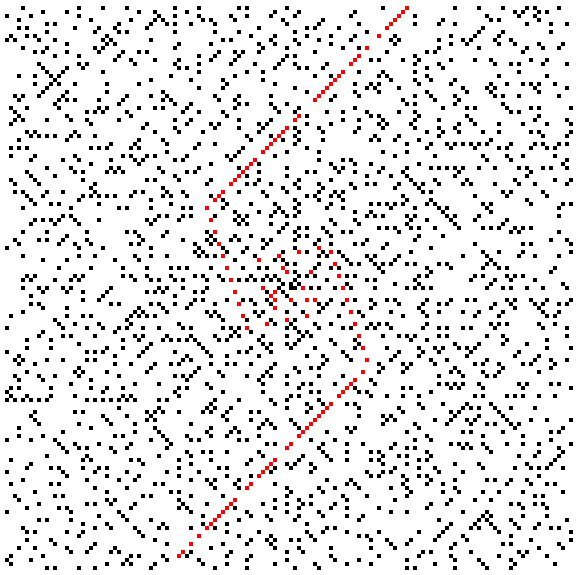
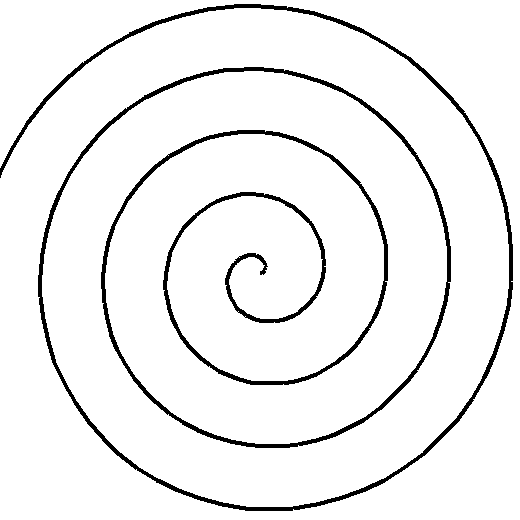
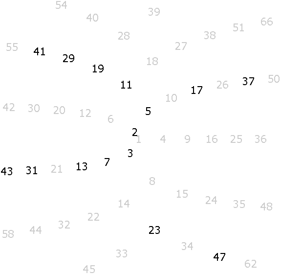
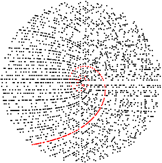
More with primes and polynomials
Other formulas
Primes and arithmetic progressions
Fermat numbers
Sophie Germain primes
Goldbach's conjecture
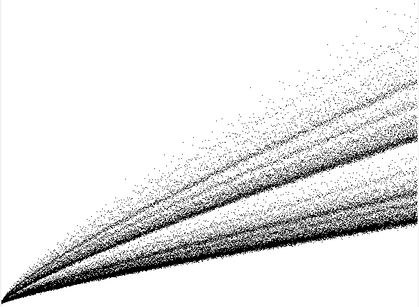
Some sums
 For example,
 Above we have ζ(1), the well-known harmonic series. We also have ζ(2) and ζ(4), whose sums were famously determined by Euler. In general, the even values, ζ(2n), always sum to some constant times π2n, whereas not too much is known about any of the odd values, except for the harmonic series.
 A remarkable fact is that the Nth partial sum of the harmonic series is nearly equal to ln(N). For instance, we have the following:
N ∑Nn = 11n ln(N) Difference 100 5.187378 4.605170 .582207 10,000 9.787606 9.210340 .577266 1,000,000 14.392727 13.815511 .577216 100,000,000 18.997896 18.420681 .577216  In other words,
 Euler then used this fact to show that the following series diverges:
 This fact gives another proof that there are infinitely many primes, since if there were only finitely many primes, then the series would have to converge. It can in fact be shown that, analogously to the harmonic series, the partial sums of this series satisfy the following:
 The constant .261497 is called the Meissel-Mertens constant.
 The constant 1.902 is called Brun's constant.**A 1994 calculation of the constant was responsible for finding a bug in the Pentium processor. See the article How Number Theory Got the Best of the Pentium Chip in the January 13, 1995 issue of Science magazine.
The Riemann hypothesis
 And there are deeper connections. For example, the prime number theorem turns out to be equivalent to the fact that the zeta function has no zeros on the line with real part -1.
Number-theoretic functions
Computing τ(n)
Let's start by computing τ(1400). We have 1400 = 23 · 52 · 7. Any divisor will include 0, 1, 2, or 3 twos, 0, 1, or 2 fives, and 0 or 1 seven. So we have 4 choices for the twos, 3 choices for the fives, and 2 choices for the sevens. There are thus 4 · 3 · 2 = 24 possible divisors in total.

Computing σ(n)
Let's compute σ(1400). Again, we have 1400 = 23 · 52 · 7. Consider the following product:
 The right hand side is exactly σ(1400); each divisor appears exactly once in the sum. On the other hand, each term on the left side can be rewritten using the geometric series formula. So we end up with
 In general, given the prime factorization n = pe11pe22 ··· pekk, we have

Computing φ(n)
 For example, to compute φ(1400), we note 1400 = 23 · 52 · 7 and compute
 As another example, to compute φ(164934), we have 164934 = 2 · 32 · 72 · 11 · 17 and so

1 2 3 4 5 6 7 8 9 10 11 12 13 14 15 16 17 18 19 20 21 22 23 24 25 26 27 28 29 30 1 2 3 4 5 6 7 8 9 10 11 12 13 14 15 16 17 18 19 20 21 22 23 24 25 26 27 28 29 30 31 32 33 1 2 … m m+1 m+2 … 2m 2m+1 2m+2 … 3m ⋮ ⋮ ⋱ ⋮ (n–1)m+1 (n–1)m+2 … nm
d Integers a with gcd(a, 10) = d φ(10/d) 1 1, 3, 7, 9 φ(10) = 4 2 2, 4, 6, 8 φ(5) = 4 5 5 φ(2) = 2 10 10 φ(1) = 1  and the latter sum must equal n as each integer from 1 through n must fall into exactly one of the sets |{a : gcd(a, n) = d}|.
Multiplicative functions
The Möbius function

Modular arithmetic
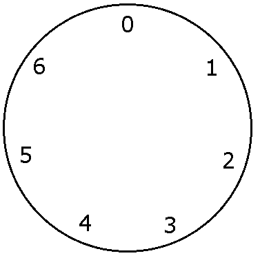
A few examples
Working with congruences
Relationship to the mod operator
Given an integer m, if we want to find the smallest positive integer k such that m ≡ k (mod n), we have k = m mod n.
An integer n is of the form ak+b if and only if n ≡ b (mod a).
Algebraic rules
These are simple rules that are easy to prove. We will use them without referring to them.


Canceling terms
Breaking things into cases
Breaking up a mod

Working with the definition
Powers
a0 a1 a2 a3 a4 a5 a6 a = 1 1 1 1 1 1 1 1 a = 2 1 2 4 1 2 4 1 a = 3 1 3 2 6 4 5 1 a = 4 1 4 2 1 4 2 1 a = 5 1 5 4 6 2 3 1 a = 6 1 6 1 6 1 6 1 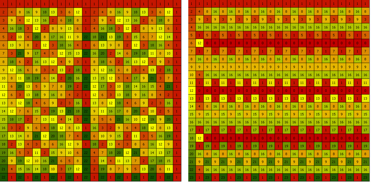

 Then we break up 5100 as 564+32+4, which is 564 · 532 · 54 or 9 · 3 · 9. This reduces to 1 modulo 11.
def mpow(b,e,n):
    prod = 1
    while e > 0:
        if e % 2 == 1:
            prod = (prod * b) % n
        e = e // 2
        b = (b*b) % n
    return prod % n
Some further examples of modular arithmetic
 The sum of the digits of the number is S = dk+dk–1+… + d1 + d0. We can see that n ≡ S (mod 3) because
 Since n and S are congruent modulo 3, whenever one is divisible by 3, the other is, too.
1000 100 10 1 – 994 98 7 0 6 2 3 1 
Fermat's little theorem
 Each binomial coefficient, (pk) with 1 < k < p, can be written as below:
 Since p is prime, no term in the denominator will cancel with p, meaning that each binomial coefficient is divisible by p and hence congruent to 0 modulo p. Thus only the ap and bp terms survive.

Euler's theorem
 And we can cancel the common terms to get 34 ≡ 1 (mod 10). We can formalize this example into a proof of Euler's theorem.
 Since each xi is relatively prime to n, we can cancel it from both sides, leaving us with aφ(n) ≡ 1 (mod n).
Formal definition and inverses
 We usually use the smallest nonnegative integer in the set to give set its name. We define ℤn to be the set {[0], [1], …, [n–1]}, with the addition and multiplication defined by [a]+[b] = [a+b] and [a] × [b] = [a × b].
Inverses
Wilson's theorem

 In general, if p is prime, then in ℤp, we can pair off everything except 1 and p–1 into inverse pairs. The numbers in each pair will cancel each other out in (p–1)!, leaving just p–1.
Solving congruences
In ordinary algebra, solving the linear equation ax = b is very useful and also very easy. Solving the congruence ax ≡ b (mod n) is also useful, but a little trickier than solving ax = b.
Procedure for solving ax ≡ b (mod n)
A few notes on finding an initial solution
 We can stop the Euclidean algorithm here as we see that the gcd will be 1. We then write
 So we have 8(3) – 23 (1) = 1 and multiplying through by 11 gives 8(33) + 23(–11) = 11. So x0 = 33 is a solution, which we can reduce mod 23 to get x0 = 10.
Examples
 We can stop the Euclidean algorithm here as we see that the gcd will be 1. Then use the extended Euclidean algorithm to get
 So we have 14(8) – 37(3) = 1 and multiplying through by 4 gives 14(32) + 37(–12) = 4. From this, we get x0 = 32 is the solution.
 In other words, they are 4, 9, 14, 19, 24, and 29.
Solving linear Diophantine equations
 for any t ∈ ℤ. Here we need some solution (x0, y0) to ax+by = c to get us started. Such a solution can be found using the extended Euclidean algorithm, trial and error, or by working with congruences. Note that there is no solution if c is not divisible by gcd(a, b).
 for any t ∈ ℤ. Each value of t gives a different solution. For instance t = 1 gives (69, –26) and t = –1 gives (–5, 2). And we can check our work: (–5, 2) is a solution because 14(–5)+37(2) = 4.
 for any t ∈ ℤ. For example, t = –2, -1, 0, 1, and 2 give (–6, 3), (–1, 1), (4, –1), (9, –3), and (14, –5) .
 for any t ∈ ℤ. However, not all solutions will make sense since neither x nor y can be negative as they represent the numbers of apples and oranges bought. So we must have 4836 + 25t ≥ 0 and –4433 – 23t ≥ 0. The first inequality can be solved to give us t ≥ –193.44. The second gives us t ≤ –192.74. So only t = –193 will give us positive values for x and y, which turn out to be x = 11 and y = 6.
A person has 5 rubies, 8 sapphires, 7 pearls, and 92 coins, while the other has 19 rubies, 14 sapphires, 2 pearls, and 4 coins. The combined worth is the same for both people. How many coins must rubies, sapphires, and pearls each be worth?
 for any t ∈ ℤ. Going back to the equation 14(1)+6(–2) = 2 and multiplying through by n = 264–5t gives 14(264–5t)+6(–528+10t) = 2(264–5t). Thus all solutions of 14r+6s–5p = 88 are of the form
 for any t, u ∈ ℤ. We are looking for positive integers, so we know that 88–2t > 0 and hence t < 44. From this and the equation for s, we get that u < –14. Note that we can make things look a little nicer by setting t = 43–x and u = –14–y. Then we have
 for x, y ≥ 0. For instance, x = y = 0 produces r = 4, s = 7, and p = 2, while x = y = 1 produces r = 6, s = 4, p = 4. Not all values of x and y will produce positive solutions, but there are infinitely many that do.
Equations with 3 or more unknowns
 for any s, t ∈ ℤ. This works provided gcd(a, b, c) ∣ d.
The Chinese remainder theorem
 where the ni are pairwise relatively prime. Then we can find a solution that is unique modulo the product n1n2 ··· nk.
 Note that gcd(5, 7) = gcd(5, 8) = gcd(7, 8) = 1, so we can use the Chinese remainder theorem. We have N = 5 · 7 · 8 = 280 along with N1 = 7 · 8 = 56, N2 = 5 · 8 = 40, and N3 = 5 · 7 = 35. We then solve the following three congruences:
 The first equation reduces to x1 ≡ 1 (mod 5), so x1 = 1. The second reduces to 5x2 ≡ 1 (mod 7), from which we get x2 = 3. The last reduces to 3x3 ≡ 1 (mod 8), from which we get x3 = 3. Then the solution is
 We can check that this works: 268 leaves a remainder of 3 when divided by 5, a remainder of 2 when divided by 7, and a remainder of 4 when divided by 8.
 We have N = 10 · 7 · 3 = 210 and N1 = 7 · 3 = 21 and N2 = 10 · 3 = 30. Because of the 0 in the last congruence, there is no need to worry about N3 and its associated congruence. We then solve the following two congruences:
 We get x1 = 1 and x2 = 4. The solution to the problem is then
 Thus the salesmen were last here together 48 days ago and will all be back 162 days from now. They are all in town together every 210 days thereafter.
Moduli that aren't relatively prime

 This turns out to have a solution of 58, which is unique modulo 60.
 The system has a unique solution modulo lcm(n1, n2, ··· , nk) if and only if ai ≡ aj (mod gcd(ni, nj)) for all i and j.
 We can't use the Chinese remainder theorem yet as the moduli are not pairwise relatively prime. But we can eliminate some of them. For instance, the first congruence says that the number of eggs is odd. But the third congruence tells us the number of eggs is of the form 4k+3, which is odd. So we can drop the first congruence.
 We then compute N = 3 · 4 · 5 · 7 = 420, N1 = 4 · 5 · 7 = 140, N2 = 3 · 5 · 7 = 105, N3 = 3 · 4 · 7 = 84. We don't need N4 because of the 0 in the last congruence. We then solve
 To get x1 = 2, x2 = 1, and x3 = 4. The solution is then

A few notes
Order
 But since the order of a was assumed to be 7, it is not possible to have a power less than the seventh power be congruent to 1. Here is a formal statement and proof of the theorem.
 So we have ar ≡ 1 (mod n), But since 0 ≤ r < k and the order of a is k, this is only possible if r = 0.
Primitive roots
Order Integers with that order modulo 13 1 1 2 12 3 3, 9 4 5, 8 6 4, 10 12 2, 6, 7, 11 
 Then order of b is thus 15, which is lcm(8, 30)/8. In general, we have the following:
So the order of b is m/k. By Theorem 5, we can also write the order of b is φ(n)/ gcd(k, φ(n)).
Finding primitive roots
from fractions import gcd

def phi(n):
    return len([x for x in range(1,n) if gcd(x,n)==1])

def order(a, n):
    if gcd(a,n) != 1:
        return -1
    c = a % n
    p = 1
    while c != 1:
        c = c*a % n
        p += 1
    return p

def prim_roots(n):
    return [a for a in range(1,n) if order(a, n)==phi(n)]
Decimal expansions
1/3 .3 1/5 .2 1/6 .16 1/7 .142856 1/11 .09 1/13 .076923 1/17 .0588235294117647 1/19 .052631578947368421 1/37 .027  The quotients 1, 4, 2, 8, 5, 7, 1, … are the digits of the decimal expansion. At each stage the remainder term from the previous step is multiplied by 10 and becomes the new dividend. Since the remainder is guaranteed to be between 0 and b–1, eventually a remainder will be repeated, causing the decimal expansion to repeat. It is interesting to note that changing the 10 to another integer d will give the base-d decimal expansion of a/b.
for i in range(n):
    print(10 * a // b)
    a = 10 * a % b
Quadratic Reciprocity
Basic properties
Euler's identity
 Now suppose a is a quadratic nonresidue. For any b = 1, 2, …, p–1, the congruence bx ≡ a (mod p) has a unique solution since p is prime, and since a is a quadratic nonresidue, we can't have x = b. As a consequence, the integers 1, 2, …, p–1 can be broken up into (p–1)/2 pairs whose products all equal a. Therefore, we have a(p–1)/2 ≡ (p–1)! (mod p) and this is congruent to -1 by Wilson's theorem.
 so -1 is a quadratic residue of any 4k+1 prime. On the other hand, for a 4k+3 prime, a similar computation results in -1, showing -1 is a quadratic nonresidue for 4k+3 primes.

Gauss's lemma
Eisenstein's lemma

 We have chosen to write all of the remainders that are larger than p/2 in a particular way. If we add up all these equations, we get
 If we then write this equation as a congruence modulo 2, we get the following
 This is because 5 and 13 are both odd an hence congruent to 1 modulo 2, and since any integer is congruent to its negative mod 2, we get that
(1+2+3+4+5+6) and 5–3+2–6–1+4 are congruent. The right side of the congruence, 3, is the number of multiples greater than p/2, which we know from Gauss's lemma is equal to (ap).
This is because 5 and 13 are both odd an hence congruent to 1 modulo 2, and since any integer is congruent to its negative mod 2, we get that
(1+2+3+4+5+6) and 5–3+2–6–1+4 are congruent. The right side of the congruence, 3, is the number of multiples greater than p/2, which we know from Gauss's lemma is equal to (ap).
 We will now write this equation as a congruence mod 2. Note that a and p are both congruent to 1 mod 2. By the argument used in the proof of Gauss's lemma, {s1, s2, …, sk} = {1, 2, …, (p–1)/2}. Since x ≡ –x (mod 2) for any integer x, we must then have s1+s2+…+sk ≡ 1+2+…+(p–1)/2 (mod 2). Thus the equation above, when written as a congruence mod 2, reduce to

The law of quadratic reciprocity

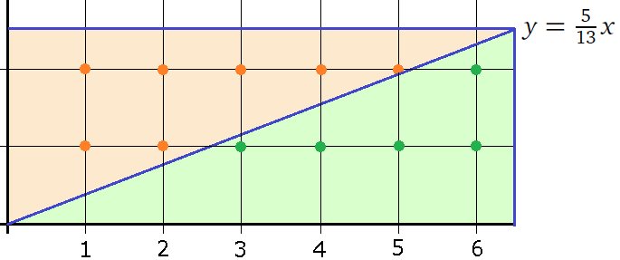


If either p or q is of the form 4k+1, then (pq) = (qp). Otherwise, (pq) = –(qp).
 So 7 is a quadratic residue of 47.
Let n > 0. Then Fn is prime if and only if 3(Fn–1)/2 ≡ –1 (mod Fn).
def pepin(n):
    f = 2**(2**n)+1
    return pow(3,(f-1)//2,f) == f-1
The Jacobi symbol
 where the symbols (api) are Legendre symbols. The Jacobi symbol has many of the same properties as the Legendre symbol. The one notable exception is that it doesn't tell us wither a is a quadratic residue or not. However, it turns out to have a number of important applications in math and cryptography.
Cryptography
Diffie-Hellman key exchange
     A B C D E F G H I J K L M N O P Q R S T U V W X Y Z
     Q W B R S E T P U M F X H V Z O K A G Y C N D J I L
Possible problems with Diffie-Hellman
RSA cryptography
 Here is an example: Suppose Alice chooses p = 13 and q = 17. Then n = pq = 221. Note also that (p–1)(q–1) = 192. Alice then chooses an e with no factors in common with 192, say e = 11. She then computes d such that de ≡ 1 (mod (p–1)(q–1)), which in our case becomes 11d ≡ 1 (mod 192). We get it by using the extended Euclidean algorithm, as follows (starting with the Euclidean algorithm):
 We can stop the Euclidean algorithm here as we see that the gcd will be 1. We then write
 Thus we have 11 · 35 – 192 · 2 = 1, so d = 35.
Possible problems with RSA
Elliptic curve cryptography
This section provides a brief introduction to elliptic curve cryptography. We will leave many mathematical details out and oversimplify some things.
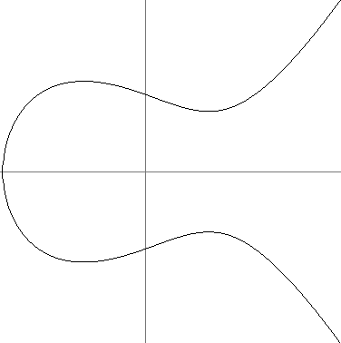
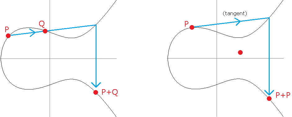
Special numbers
Perfect numbers and Mersenne primes
The formula for computing σ tells us that σ(2n–1) = 2n–1, and we have σ(2n–1) = 2n since 2n–1 is prime. Putting this together gives us σ(k) = 2k.
 Since k is perfect, σ(k) = 2k = 2nm, and so we have
 Thus 2n–1 is a divisor of 2nm. By Euclid's lemma, since gcd(2n–1, 2n) = 1, we must have 2n–1 ∣ m. So we can write (2n–1)j = m for some integer j. Plugging this in to the equation above and simplifying gives 2nj = σ(m).
There are quite a few others. See the Wikipedia page on perfect numbers for more.
Finding Mersenne primes
There is a reason why the largest known primes are all Mersenne primes: there is an easy test to tell if a Mersenne number is prime:
 As S6 is congruent to 0 mod 127, we conclude that 27–1 is a Mersenne prime.
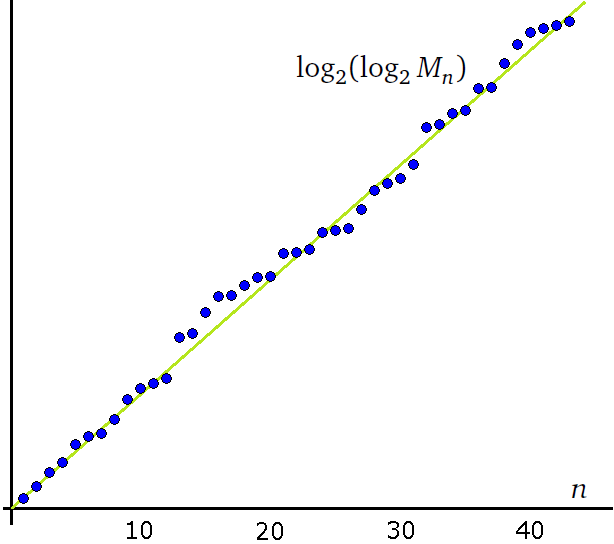
Pythagorean triples
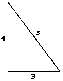
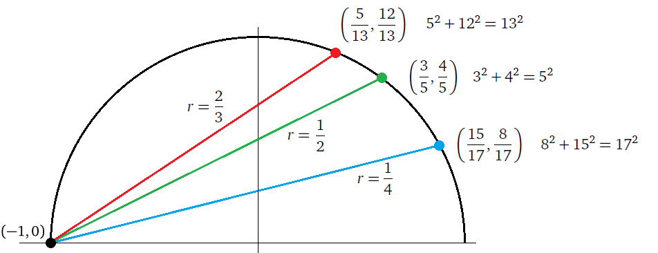
 From this, we get x = 1–r21+r2 and plugging back into the line equation gives y = 2r1+r2. Each value of r gives a different rational point (x, y) on the curve. If we write r = m/n for some integers m and n, and convert the rational point into a triple, we get the desired formulas a = n2–m2, b = 2mn, c = n2+m2.
See the Wikipedia page on Pythagorean triples for more properties.
Fermat's last theorem
So we have seen that there are infinitely many integer solutions to x2+y2 = z2. What about x3+y3 = z3 or x4+y4 = z4? One of the most famous stories from math concerns these equations. Fermat wrote in the margin of a copy of Diophantus' Arithmetica that he had a proof that xn+yn = zn has no integer solutions and said he couldn't include it because the book's margin was too small to hold the proof. People tried for the next 350 years to prove it before it was finally resolved by Andrew Wiles in the 1990s.
Primality testing and factoring
Primality testing
def is_prime(n):
    if n in [2,3,5,7,11,13,17,19,23]:
        return True
    if n==0 or n==1 or n%2==0 or n%3==0:
        return False
    d = 5
    step = 2
    stop = n**.5
    while d <= stop:
        if n % d == 0:
            return False
        d += step
        step = 4 if step == 2 else 2
    return True
prime running time in seconds 100000000003 0.08 1000000000039 0.22 10000000000037 0.91 100000000000031 2.47 1000000000000037 8.14 10000000000000061 24.54 Probabilistic primality tests
 By Fermat's little theorem, an–1–1 = 0, so one of the factors of the right side must be 0. Hence once of those congruences must hold.
def miller_rabin(n, tries=10):
    s = 0
    t = n-1
    while t%2 == 0:
        t //= 2
        s += 1

    for i in range(tries):
        a = random.randint(2,n-2)
        b = pow(a,t,n)
        if b!=1 and b!=n-1:
            for j in range(s):
                b = pow(b,2,n)
                if b == n-1:
                    break
            else:
                return False
    return True
Factoring
Fermat's method
3462–119143 = 573
3472–119143 = 1266
3482–119143 = 1961
3492–119143 = 2658
3502–119143 = 3357
3512–119143 = 4058
3522–119143 = 4761 = 692.
from math import floor, ceil

def is_perfect_square(n):
    return abs(n**.5 - floor(n**.5)) < 1e-14

def fermat_factor(n):
    x = ceil(n**.5)
    y = x*x - n
    while not is_perfect_square(y):
        x += 1
        y = x*x - n
    return (x-floor(y**.5), x+floor(y**.5))
The Pollard rho method
 Notice that x4–x0 = 26–1 is divisible by 13. Also, x5–x1 = 195 and x6–x2 = 130 are divisible by 13, and in general, xm+4–xm is divisible by 13 for any m ≥ 4. Further, notice that x7–x1 = 102, x8–x2 = 204, x9–x1 = 119, etc. are all divisible by 17. This sort of thing will always happen for the divisors of an integer. This suggests a way to find factors of an integer n: Look at the sequence of iterates of x2+1 and look at gcd(n, xk–xj). Eventually this should (but not always) lead to a factor of n.
from random import randint
from fractions import gcd

def pollard_rho(n):
    g = n
    while g == n:
        c = randint(1,n-3)
        s = randint(0,n-1)
        u = v = s
        f = lambda x:(x*x+c) % n

        g = 1
        while g == 1:
            u = f(u)
            v = f(f(v))
            g = gcd(u-v,n)
    return g
Appendix of useful algebra
 A particularly useful special case of this is y = 1.
 Recall that (nk) is called a binomial coefficient and is often read as “n choose k”. We have
 For example,
 Note that the number of terms in the numerator and denominator of the reduced form is always the same. Binomial coefficients can also be read off of Pascal's triangle, where (nk) is the entry in row n, column k of the triangle (where we start counting rows and columns at index 0 instead of 1).
Bibliography
