An Intuitive Guide to Numerical Methods
© 2019 Brian Heinold Here is a pdf version of the book.
One thing that is missing here is linear algebra. Most of my students hadn't yet taken linear algebra, so it wasn't something I covered.
I have included Python code for many of the methods. I find that sometimes it is easier for me to understand how a numerical method works by looking at a program. Python is easy to read, being almost like pseudocode (with the added benefit that it actually runs). However, everything has been coded for clarity, not for efficiency or robustness. In real-life there are lots of edge cases that need to be checked, but checking them clutters the code, and that would defeat the purpose of using the code to illustrate the method. In short, do not use the code in this book for anything important.
There are a few hundred exercises, mostly of my own creation. They are all grouped together in Chapter 7.
If you see anything wrong (including typos), please send me a note at heinold@msmary.edu.
Equations like 3x+4 = 7 or x2–2x+9 = 0 can be solved using high school algebra. Equations like 2x3+4x2+3x+1 = 0 or x4+x+1 = 0 can be solved by some more complicated algebra.
But the equation x5–x+1 = 0 cannot be solved algebraically. There are no algebraic techniques that will give us an answer in terms of anything familiar. If we need a solution to an equation like this, we use a numerical method, a technique that will give us an approximate solution.
Here is a simple example of a numerical method that estimates √5: Start with a guess for √5, say x = 2 (since √4 = 2 and 5 is pretty close to 4). Then compute
This is what a numerical method is—a process that produces approximate solutions to some problem. The process is often repeated like this, where approximations are plugged into the method to generate newer, better approximations. Often a method can be run over and over until a desired amount of accuracy is obtained.
It is important to study how well the method performs. There are a number of questions to ask: Does it always work? How quickly does it work? How well does it work on a computer?
Now, in case a method to find the square root seems silly to you, consider the following: How would you find the square root of a number without a calculator? Notice that this method allows us to estimate the square root using only the basic operations of addition and division. So you could do it by hand if you wanted to. In fact it's called the Babylonian method, or Hero's method, as it was used in Babylon and ancient Greece. It used to be taught in school until calculators came along.**Calculators themselves use numerical methods to find square roots. Many calculators use efficient numerical methods to compute ex and ln x and use the following identity to obtain √x from ex and ln x:
Most numerical methods are implemented on computers and calculators, so we need to understand a little about how computers and calculators do their computations.
Computer hardware cannot not represent most real numbers exactly. For instance, π has an infinite, non-repeating decimal expansion that would require an infinite amount of space to store. Most computers use something called floating-point arithmetic, specifically the IEEE 754 standard. We'll just give a brief overview of how things work here, leaving out a lot of details.
The most common way to store real numbers uses 8 bytes (64 bits). It helps to think of the number as written in scientific notation. For instance, write 25.394 as 2.5394 × 10². In this expression, 2.5394 is called the mantissa. The 2 in 102 is the exponent. Note that instead of a base 10 exponent, computers, which work in binary, use a base 2 exponent. For instance, .3 is written as 1.2 × 2–2.
Of the 64 bits, 53 are used to store the mantissa, 11 are for the exponent, and 1 bit is used for the sign (+ or –). These numbers actually add to 65, not 64, as a special trick allows an extra bit of info for the mantissa. The 53 bits for the mantissa allow for about 15 digits of precision. The 11 bits for the exponent allow numbers to range from as small as 10–307 to as large as 10308.
The precision limits mean that we cannot distinguish 123.000000000000007 from 123.000000000000008. However, we would be able to distinguish .000000000000000007 and .000000000000000008 because those numbers would be stored as 7 × 10–18 and 8 × 10–18. The first set of numbers requires more than 15 digits of precision, while the second pair requires very little precision.
Also, doing something like 1000000000 + .00000004 will just result in 1000000000 as the 4 falls beyond the precision limit.
When reading stuff about numerical methods, you will often come across the term machine epsilon. It is defined as the difference between 1 and the closest floating-point number larger than 1. In the 64-bit system described above, that value is about 2.22 × 10⁻¹⁶. Machine epsilon is a good estimate of the limit of accuracy of floating-point arithmetic. If the difference between two real numbers is less than machine epsilon, it is possible that the computer would not be able to tell them apart.
One interesting thing is that many numbers, like .1 or .2, cannot be represented exactly using IEEE 754. The reason for this is that computers store numbers in binary (base 2), whereas our number system is decimal (base 10), and fractions behave differently in the two bases. For instance, converting .2 to binary yields .00110011001100…, an endlessly repeating expansion. Since there are only 53 bits available for the mantissa, any repeating representation has to be cut off somewhere.**It's interesting to note that the only decimal fractions that have terminating binary expansions are those whose denominators are powers of 2. In base 10, the only terminating expansions come from denominators that are of the form 2j5k. This is because the only proper divisors of 10 are 2 and 5. This is called roundoff error. If you convert the cut-off representation back to decimal, you actually get .19999999999999998.
If you write a lot of computer programs, you may have run into this problem when printing numbers. For example, consider the following simple Python program:
We would expect it to print out .3, but in fact, because of roundoff errors in both .2 and .1, the result is 0.30000000000000004.
Actually, if we want to see exactly how a number such as .1 is represented in floating-point, we can do the following:
The result is 0.1000000000000000055511151231257827021181583404541015625000000000000000.
This number is the closest IEEE 754 floating-point number to .1. Specifically, we can write .1 as .8 × 2–3, and in binary, .8 is the has a repeating binary expansion .110011001100…. That expansion gets cut off after 53 bits and that eventually leads to the strange digits that show up around the 18th decimal place.
One big problem with this is that these small roundoff errors can accumulate, or propagate. For instance, consider the following Python program:
Here is something else that can go wrong: Try computing the following:
The exact answer should be .1, but the program gives 0.11102230246251565, only correct to one decimal place. The problem here is that we are subtracting two numbers that are very close to each other. This causes all the incorrect digits beyond the 15th place in the representation of .1 to essentially take over the calculation. Subtraction of very close numbers can cause serious problems for numerical methods and it is usually necessary to rework the method, often using algebra, to eliminate some subtractions.
This is sometimes called the Golden rule of numerical analysis: don't subtract nearly equal numbers.
The 64-bit storage method above is called IEEE 754 double-precision (this is where the data type double in many programming languages gets its name). There is also 32-bit single-precision and 128-bit quadruple-precision specified in the IEEE 754 standard.
Single-precision is the float data type in many programming languages. It uses 24 bits for the mantissa and 8 for the exponent, giving about 6 digits of precision and values as small as 10–128 to as large as 10127. The advantages of single-precision over double-precision are that it uses half as much memory and computations with single-precision numbers often run a little more quickly. On the other hand, for many applications these considerations are not too important.
Quadruple-precision is implemented by some programming languages.**There is also an 80-bit extended precision method on x86 processors that is accessible via the long double type in C and some other languages. One big difference between it and single- and double-precision is that the latter are usually implemented in hardware, while the former is usually implemented in software. Implementing in software, rather than having specially designed circuitry to do computations, results in a significant slowdown.
For most scientific calculations, like the ones we are interested in a numerical methods course, double-precision will be what we use. Support for it is built directly into hardware and most programming languages. If we need more precision, quadruple-precision and arbitrary precision are available in libraries for most programming languages. For instance, Java's BigDecimal class and Python's Decimal class can represent real numbers to very high precision. The drawback to these is that they are implemented in software and thus are much slower than a native double-precision type. For many numerical methods this slowdown makes the methods too slow to use.
See the article, “What Every Computer Scientist Should Know About Floating-Point Arithmetic” at http://docs.oracle.com/cd/E19957-01/806-3568/ncg_goldberg.html for more details about floating-point arithmetic.
Solving equations is of fundamental importance. Often many problems at their core come down to solving equations. For instance, one of the most useful parts of calculus is maximizing and minimizing things, and this usually comes down to setting the derivative to 0 and solving.
As noted earlier, there are many equations, such as x5–x+1 = 0, which cannot be solved exactly in terms of familiar functions. The next several sections are about how to find approximate solutions to equations.
The bisection method is one of the simpler root-finding methods. If you were to put someone in a room and tell them not to come out until they come up with a root-finding method, the bisection method is probably the one they would come up with.
Here is the idea of how it works. Suppose we want to find a root of f(x) = 1–2x–x5. First notice that f(0) = 1, which is above the x-axis and f(1) = –2, which is below the axis. For the function to get from 1 to –2, it must cross the axis somewhere, and that point is the root.**This is common sense, but it also comes from the Intermediate Value Theorem. So we know a root lies somewhere between x = 0 and x = 1. See the figure below.
Next we look at the midpoint of 0 and 1, which is x = .5 (i.e., we bisect the interval) and check the value of the function there. It turns out that f(.5) = –0.03125. Since this is negative and f(0) = 1 is positive, we know that the function must cross the axis (and thus have a root) between x = 0 and x = .5. We can then bisect again, by looking at the value of f(.25), which turns out to be around .499. Since this is positive and f(.5) is negative, we know the root must be between x = .25 and x = .5. We can keep up this bisection procedure as long as we like, and we will eventually zero in on the location of the root. Shown below is a graphical representation of this process.
In general, here is how the bisection method works: We start with values a and b such that f(a) and f(b) have opposite signs. If f is continuous, then we are guaranteed that a root lies between a and b. We say that a and b bracket a root.
We then compute f(m), where m = (a+b)/2. If f(m) and f(b) are of opposite signs, we set a = m; if f(m) and f(a) are of opposite signs, we set b = m. In the unlikely event that f(m) = 0, we stop because we have found a root. We then repeat the process again and again until a desired accuracy is reached. Here is how we might code this in Python:
For simplicity, we have ignored the possibility that f(m) = 0. Notice also that an easy way to check if f(a) and f(m) are of opposite signs is to check if f(a)f(m) < 0. Here is how we might call this function to do 20 bisection steps to estimate a root of x2–2:
In Python, lambda creates an anonymous function. It's basically a quick way to create a function that we can pass to our bisection function.
Let a0 and b0 denote the starting values of a and b. At each step we cut the previous interval exactly in half, so after n steps the interval has length (b0–a0)/2n. At any step, our best estimate for the root is the midpoint of the interval, which is no more than half the length of the interval away from the root, meaning that after n steps, the error is no more than (b0–a0)/2n+1.
For example, if a0 = 0, b0 = 1, and we perform n = 10 iterations, we would be within 1/211 ≈ .00049 of the actual root.
If we have a certain error tolerance ε that we want to achieve, we can solve (b0–a0)/2n+1 = ε for n to get
In the world of numerical methods for solving equations, the bisection method is very reliable, but very slow. We essentially get about one new correct decimal place for every three iterations (since log2(10) ≈ 3). Some of the methods we will consider below can double and even triple the number of correct digits at every step. Some can do even better. But this performance comes at the price of reliability. The bisection method, however slow it may be, will usually work.
However, it will miss the root of something like x2 because that function is never negative. It can also be fooled around vertical asymptotes, where a function may change from positive to negative but have no root, such as with 1/x near x = 0.
The false position method is a lot like the bisection method. The difference is that instead of choosing the midpoint of a and b, we draw a line between (a, f(a)) and (b, f(b)) and see where it crosses the axis. In particular, the crossing point can be found by finding the equation of the line, which is y–f(a) = f(b)–f(a)b–a(x–a), and setting y = 0 to get its intersection with the x axis. Solving and simplifying, we get
Try the following experiment: Pick any number. Take the cosine of it. Then take the cosine of your result. Then take the cosine of that. Keep doing this for a while. On a TI calculator, you can automate this process by typing in your number, pressing enter, then entering cos(Ans) and repeatedly pressing enter. Here's a Python program to do this along with its output:
We can see that the numbers seem to be settling down around .739. If we were to carry this out for a few dozen more iterations, we would eventually get stuck at (to 15 decimal places) 0.7390851332151607. And we will eventually settle in on this number no matter what our initial value of x is.
What is special about this value, .739…, is that it is a fixed point of cosine. It is a value which is unchanged by the cosine function; i.e., cos(.739…) = .739…. Formally, a fixed point of a function g(x) is a value p such that g(p) = p. Graphically, it's a point where the graph crosses the line y = x. See the figure below:
Some fixed points have the property that they attract nearby points towards them in the sort of iteration we did above. That is, if we start with some initial value x0, and compute g(x0), g(g(x0)), g(g(g(x0))), etc., those values will approach the fixed point. The point .739… is an attracting fixed point of cos x.
Other fixed points have the opposite property. They repel nearby points, so that it is very hard to converge to a repelling fixed point. For instance, g(x) = 2 cos x has a repelling fixed point at p = 1.02985…. If we start with a value, say x = 1, and iterate, computing g(1), g(g(1)), etc., we get 1.08, .94, 1.17, .76, 1.44, numbers which are drifting pretty quickly away from the fixed point.
Here is a way to picture fixed points: Imagine a pendulum rocking back and forth. This system has two fixed points. There is a fixed point where the pendulum is hanging straight down. This is an attracting state as the pendulum naturally wants to come to rest in that position. If you give it a small push from that point, it will soon return back to that point. There is also a repelling fixed point when the pendulum is pointing straight up. At that point you can theoretically balance the pendulum, if you could position it just right, and that fixed point is repelling because just the slighted push will move the pendulum from that point. Phenomena in physics, weather, economics, and many other fields have natural interpretations in terms of fixed points.
We can visualize the fact that the fixed point of cos x is attracting by using something called a cobweb diagram. Here is one:
In the diagram above, the function shown is g(x) = cos(x), and we start with x0 = .4. We then plug that into the function to get g(.4) = .9210…. This is represented in the cobweb diagram by the line that goes from the x-axis to the cosine graph. We then compute g(g(.4)) (which is g(.9210…)). What we are doing here is essentially taking the previous y-value, turning it into an x-value, and plugging that into the function. Turning the y-value into an x-value is represented graphically by the horizontal line that goes from our previous location on the graph to the line y = x. Then plugging in that value into the function is represented by the vertical line that goes down to the graph of the function.
We then repeat the process by going over to y = x, then to y = cos(x), then over to y = x, then to y = cos(x), etc. We see that the iteration is eventually sucked into the fixed point.
Here is an example of a repelling fixed point, iterating g(x) = 1–2x–x5.
The key to whether a fixed point p is attracting or repelling turns out to be the value of g′(p), the slope of the graph at the fixed point. If |g′(p)| < 1 then the fixed point is attracting. If |g′(p)| > 1, the fixed point is repelling.**This result is sometimes called the Banach fixed point theorem and can be formally proved using the Mean Value Theorem. Graphically, if the function is relatively flat near the fixed point, the lines in the cobweb diagram will be drawn in towards the fixed point, whereas if the function is steeply sloped, the lines will be pushed away. If |g′(p)| = 1, a more sophisticated analysis is needed to determine the point's behavior, as it can be (slowly) attracting, (slowly) repelling, possibly both, or divergent.
The value of |g′(p)| also determines the speed at which the iterates converge towards the fixed point. The closer |g′(p)| is to 0, the faster the iterates will converge. A very flat graph, for instance, will draw the cobweb diagram quickly into the fixed point.
One caveat here is that an attracting fixed point is only guaranteed to attract nearby points to it, and the definition of “nearby” will vary from function to function. In the case of cosine, “nearby” includes all of ℝ, whereas with other functions “nearby” might mean only on a very small interval.
The process described above, where we compute g(x0), g(g(x0)), g(g(g(x0))), … is called fixed point iteration. It can be used to find an (attracting) fixed point of f. We can use this to find roots of equations if we rewrite the equation as a fixed point problem.
For instance, suppose we want to solve 1–2x–x5 = 0. We can rewrite this as a fixed point problem by moving the 2x over and dividing by 2 to get (1–x5)/2 = x. It is now of the form g(x) = x for g(x) = (1–x5)/2. We can then iterate this just like we iterated cos(x) earlier.
We start by picking a value, preferably one close to a root of 1–2x–x5. Looking at a graph of the function, x0 = .5 seems like a good choice. We then iterate. Here is result of the first 20 iterations:
We see that the iterates pretty quickly settle down to about .486389035934543.
On a TI calculator, you can get the above (possibly to less decimal places) by entering in .5, pressing enter, then entering in There are a couple of things to note here about the results. First, the value of |g′(p)| is about .14, which is pretty small, so the convergence is relatively fast. We add about one new correct digit with every iteration. We can see in the figure below that the graph is pretty flat around the fixed point. If you try drawing a cobweb diagram, you will see that the iteration gets pulled into the fixed point very quickly.
Second, the starting value matters. If our starting value is larger than about 1.25 or smaller than -1.25, we are in the steeply sloped portion of the graph, and the iterates will be pushed off to infinity. We are essentially outside the realm of influence of the fixed point.
Third, the way we rewrote 1–2x–x5 = 0 was not the only way to do so. For instance, we could instead move the x5 term over and take the fifth root of both sides to get 5√1–2x = x. However, this would be a bad choice, as the derivative of this function at the fixed point is about -7, which makes the point repelling. A different option would be to write 1 = 2x+x5, factor out an x and solve to get 1x4+2 = x. For this iteration, the derivative at the fixed point is about –.11, so this is a good choice.
Here is a clever way to turn f(x) = 0 into a fixed point problem: divide both sides of the equation by –f′(x) and then add x to both sides. This gives
Iterating x–f(x)f′(x) to find a root of f is known as Newton's method.**It is also called the Newton-Raphson method. As an example, suppose we want a root of f(x) = 1–2x–x5. To use Newton's method, we first compute f′(x) = –2–4x5. So we will be iterating
After just a few iterations, Newton's method has already found as many digits as possible in double-precision floating-point arithmetic.
To get this on a TI calculator, put in .5, press enter, then put in The figure below shows a nice way to picture how Newton's method works. The main idea is that if x0 is sufficiently close to a root of f, then the tangent line to the graph at (x0, f(x0)) will cross the x-axis at a point closer to the root than x0.
What we do is start with an initial guess for the root and draw a line up to the graph of the function. Then we follow the tangent line down to the x-axis. From there, we draw a line up to the graph of the function and another tangent line down to the x-axis. We keep repeating this process until we (hopefully) get close to a root. It's a kind of slanted and translated version of a cobweb diagram.
This geometric process helps motivate the formula we derived for Newton's method. If x0 is our initial guess, then (x0, f(x0)) is the point where the vertical line meets the graph. We then draw the tangent line to the graph. The equation of this line is y–f(x0) = f′(x0)(x–x0). This line crosses the x-axis when y = 0, so plugging y = 0 and solving for x, we get that the new x value is x0–f(x0)f′(x0).
There are a few things that can go wrong with Newton's method. One thing is that f′(x) might be 0 at a point that is being evaluated. In that case the tangent line will be horizontal and will never meet the x-axis (note that the denominator in the formula will be 0). See below on the left. Another possibility can be seen with f(x) = 3√x–1. Its derivative is infinite at its root, x = 1, which has the effect of pushing tangent lines away from the root. See below on the right.
Also, just like with fixed-point iteration, if we choose a starting value that is too far from the root, the slopes of the function might push us away from the root, never to come back, like in the figure below:
There are stranger things that can happen. Consider using Newton's method to find a root of f(x) = 3√(3–4x)/x.
After a fair amount of simplification, the formula x–f(x)f′(x) for this function becomes 4x(1–x). Now, a numerical method is not really needed here because it is easy to see that the function has a root at x = 3/4 (and this is its only root). But it's interesting to see how the method behaves. One thing to note is that the derivative goes vertical at x = 3/4, so we would expect Newton's method to have some trouble. But the trouble it has is surprising.
Here are the first 36 values we get if we use a starting value of .4. There is no hint of this settling down on a value, and indeed it won't ever settle down on a value.
But things are even stranger. Here are the first 10 iterations for two very close starting values, .400 and .401:
We see these values very quickly diverge from each other. This is called sensitive dependence on initial conditions. Even if our starting values were vanishingly close, say only 10–20 apart, it would only take several dozen iterations for them to start to diverge. This is a hallmark of chaos. Basically, Newton's method is hopeless here.
Finally, to show a little more of the interesting behavior of Newton's method, the figure below looks at iterating Newton's method on x5–1 with starting values that could be real or complex numbers. Each point in the picture corresponds to a different starting value, and the color of the point is based on the number of iterations it takes until the iterates get within 10–5 of each other.
The five light areas correspond to the five roots of x5–1 (there is one real root at x = 1 and four complex roots). Starting values close to those roots get sucked into those roots pretty quickly. However, points in between the two roots bounce back and forth rather chaotically before finally getting trapped by one of the roots. The end result is an extremely intricate picture. It is actually a fractal in that one could continuously zoom in on that figure and see more and more intricate detail that retains the same chaining structure as in the zoomed-out figure.
We can use Newton's method to derive a method for estimating square roots. The trick is to find an appropriate function to apply Newton's method to. The simplest possibility is f(x) = x2–2. Its roots are ±√2. We have f′(x) = 2x and so the Newton's method formula is
The numerical methods we have examined thus far try to approximate a root r of a function f by computing approximations x1, x2, …, xn, which are hopefully getting closer and closer to r. We can measure the error at step i with |xi–r|, which is how far apart the approximation is from the root.
Suppose we are using FPI to estimate a solution of x3+x–1 = 0. To four decimal places, a solution turns out to be x = .6823. One way to rewrite the problem as a fixed-point problem is to write x(x2+1)–1 = 0 and solve for x to get x = 1/(x2+1). Let's start with x0 = 1 and iterate. Below are the iterates x1 through x10 along with their corresponding errors (how far off they are from .6823):
The third column is the ratio of successive errors. If we look carefully at the errors, it looks like each error is roughly 2/3 of the previous error, and the ratio ei+1/ei bears that out. In fact, after enough iterations it ends up being true that ei+1 ≈ .635 ei. When the errors go down by a nearly constant factor at each step like this, we have what is called linear convergence.
For some methods, like Newton's method, the error can go down at a faster than constant rate. For instance, if we apply Newton's method to the same problem as above, starting with x0 = 1, we get the following sequence of errors:
The errors are going down at a faster than linear rate. It turns out that they are going down roughly according to the rule ei+1 ≈ .854 e2i. This is an example of quadratic convergence.
Formally, if limi → ∞ei+1ei = s and 0 < s < 1, the method is said to converge linearly.**If s = 0, the convergence will be faster than linear. If limi → ∞ei+1e2i = s and 0 < s < 1, the method is said to converge quadratically. Cubic, quartic, etc. convergence are defined similarly. The exponent in the denominator is the key quantity of interest. It is called the order of convergence. (The order of linear convergence is 1, the order of quadratic convergence is 2, etc.)
An order of convergence greater than 1 is referred to as superlinear.
Let's examine the difference between linear and quadratic convergence: Suppose we have linear convergence of the form ei+1 ≈ .1ei. Each error is about 10% of the previous, so that if for example, e1 = .1, then we have
We add about one new decimal place of accuracy with each iteration. If we had a larger constant, say ei+1 = .5ei, then the errors would go down more slowly, but we would still add about one new decimal place of accuracy every couple of iterations.
On the other hand, suppose we have quadratic convergence of the form ei+1 ≈ e2i. If we start with e1 = .1, then we have
So we actually double the number of correct decimal places of accuracy at each step. So there is a big difference between linear and quadratic convergence. For the linear convergence described above, it would take 1000 iterations to get 1000 decimal places of accuracy, whereas for the quadratic convergence described above, it would take about 10 iterations (since 210 = 1024).
Similarly, cubic convergence roughly triples the number of correct decimal places at each step, quartic quadruples it, etc.
Suppose we are solving f(x) = 0 and that f′ and f″ exist and are continuous. Then the following hold:
In the above, “close to r” formally means that there is some interval around r for which if the initial guess falls in that interval, then the iterates will converge to r. The formal term for this is local convergence. The size of that interval varies with the function.
In summary, if a few assumptions are met, then we know that FPI converges linearly with rate |g′(r)|, bisection converges linearly with rate .5, and Newton's method converges quadratically (at simple roots).
And those assumptions can't entirely be ignored. For instance, f(x) = √x has a root at x = 0, and f″(0) does not exist. For this function, Newton's method turns out to converge very slowly to the root at 0, not quadratically.
There are generalizations of Newton's method that converge even more quickly. For instance, there is Halley's method, which involves iterating
One weakness of Newton's method is that it requires derivatives. This is usually not a problem, but for certain functions, getting and using the derivative might be inconvenient, difficult, or computationally expensive. The secant method uses the same ideas from Newton's method, but it approximates the derivative (slope of the tangent line) with the slope of a secant line.
Remember that the derivative of a function f at a point x is the slope of the tangent line at that point. The definition of the derivative, given by f′(x) = limh → 0f(x+h)–f(x)x+h, is gotten by approximating the slope of that tangent line by the slopes of secant lines between x and a nearby point x+h. As h gets smaller, x+h gets closer to x and the secant lines start to look more like tangent lines. In the figure below a secant line is shown in red and the tangent line in green.
The formula we iterate for Newton's method is
As an example, let's use the secant method to estimate a root of f(x) = 1–2x–x5. Since the formula needs two previous iterations, we will need two starting values. For simplicity, we'll pick x0 = 2 and x1 = 1. We have f(x0) = –35 and f(x1) = –2. We then get
We can see that this converges quickly, but not as quickly as Newton's method. By approximating the derivative, we lose some efficiency. Whereas the order of convergence of Newton's method is usually 2, the order of convergence of the secant method is usually the golden ratio, φ = 1.618….**Note we are only guaranteed converge if we are sufficiently close to the root. We also need the function to be relatively smooth—specifically, f″ must exist and be continuous. Also, the root must be a simple root (i.e. of multiplicity 1). Function are pretty flat near a multiple root, which makes it slow for tangent and secant lines to approach the root.
Here is a simple implementation of the secant method in Python:
Here is how we might call this to estimate a solution to x5–x+1 = 0 correct to within 10–10:
In the function, a and b are used for xn–1 and xn in the formula. The loop runs until either f(b) is 0 or the difference between two successive iterations is less than some (small) tolerance. The default tolerance is 10–10, but the caller can specify a different tolerance. The assignment line sets Our implementation is simple, but it is not very efficient or robust. For one thing, we recompute f(b) (which is f(xn)) at each step, even though we already computed it when we did f(a) (which is f(xn–1) at the previous step. A smarter approach would be to save the value. Also, it is quite possible for us to get caught in an infinite loop, especially if our starting values are poorly chosen. See Numerical Recipes for a faster and safer implementation.
A close relative of Newton's method and the secant method is to iterate the formula below:
Muller's method is a generalization of the secant method. Recall that Newton's method involves following the tangent line down to the x-axis. That point where the line crosses the axis will often be closer to the root than the previous point. The secant method is similar except that it follows a secant line down to the axis. What Muller's method does is it follows a parabola down to the axis. Whereas a secant line approximates the function via two points, a parabola uses three points, which can give a closer approximation.
Here is the formula for Muller's (where fi denotes f(xi) for any integer i):
Inverse quadratic interpolation is a relative of Muller's method. Like Muller's, it uses a parabola, but it approximates f–1 instead of f. This is essentially the same as approximating f by the inverse of a quadratic function. After some work (which we omit), we get the following iteration:
Both Muller's method and inverse quadratic interpolation have an order of convergence of about 1.839.**Like with the secant method, this result holds for starting values near a simple root, and the function must be relatively smooth. Note also that the order of the secant method, 1.618…, is the golden ratio, related to the Fibonacci numbers. The order of Muller's and IQI, 1.839…, is the tribonacci constant, related to the tribonacci numbers, defined by the recurrence xn+1 = xn + xn–1 + xn–2. That number is the solution to x3 = x2+x+1, whereas the golden ratio is the solution to x2 = x+1.
Recall that we have a and b with f(a) and f(b) of opposite signs, like in the bisection method, we say a root is bracketed by a and b. That is, the root is contained inside that interval.
Brent's method is one of the most widely used root-finding methods. You start by giving it a bracketing interval. It then uses a combination of the bisection method and inverse quadratic interpolation to find a root in that interval. In simple terms, Brent's method uses inverse quadratic interpolation unless it senses something is going awry (like an iterate leaving the bracketing interval, for example), then it switches to the safe bisection method for a bit before trying inverse quadratic interpolation again. In practice, it's a little more complicated than this. There are a number of special cases built into the algorithm. It has been carefully designed to ensure quick, guaranteed convergence in a variety of situations. It converges at least as fast as the bisection method and most of the time is better, converging superlinearly.
There are enough special cases to consider that the description of the algorithm becomes a bit messy. So we won't present it here, but a web search for Brent's method will turn up a variety of resources.
Ridder's method is a variation on bisection/false position that is easy to implement and works fairly well. Numerical Recipes recommends it as an alternative to Brent's method in many situations.
The method starts out with a and b, like in the bisection method, where one of f(a) and f(b) is positive and the other is negative. We then compute the midpoint m = (a+b)/2 and the expression
This equation gives us an improvement over the bisection method, which uses m as its estimate, leading to quadratic convergence. It is, however, slower than Newton's method, as it requires two new function evaluations at each step as opposed to only one for Newton's method. But it is more reliable than Newton's method.
There is an algorithm called Aitken's Δ2 method that can take a slowly converging sequence of iterates and speeds things up. Given a sequence {xn} create a new sequence {yn} defined as below:
Treating this as an equation and solving for r gives the formula above (after a fair bit of algebra). Here is a Python function that displays an FPI sequence and the sped up version side by side.
Here are the first few iterations we get from iterating cos x.
The fixed point of cos x is .73908 to five decimal places and we can see that after 10 iterations, the sped-up version is correct to that point. On the other hand, it takes the regular FPI about 20 more iterations to get to that point (at which point the sped-up version is already correct to 12 places).
The root-finding methods considered in previous sections can be used to find roots of all sorts of functions. But probably the most important and useful functions are polynomials. There are a few methods that are designed specifically for finding roots of polynomials. Because they are specifically tailored to one type of function, namely polynomials, they can be faster than a method that has to work for any type of function. An important method is Laguerre's method. Here is how it works to find a root of a polynomial p:
Pick a starting value x0. Compute G = p′(x0)p(x0) and H = G2–p″(x0)p(x0). Letting n be the degree of the polynomial, compute
Laguerre's method actually comes from writing the polynomial in factored form p(x) = c(x–r1)(x–r2)…(x–rn). If we take the logarithm of both sides and use the multiplicative property of logarithms, we get
Now, for a given value of x, |x–ri| represents the distance between x and ri. Suppose we are trying to estimate r1. Once we get close to r1, it might be true that all the other roots will seem far away by comparison, and so in some sense, they are all the same distance away, at least in comparison to the distance from r1. Laguerre's method suggests that we pretend this is true and assume |x–r2| = |x–r3| = … = |x–rn|. If we do this, the expressions for G and H above simplify considerably, and we get an equation that we can solve. In particular, let a = |x–r1| and b = |x–r2| = |x–r3| = … = |x–rn|. Then the expressions for G and H simplify into
Laguerre's method works surprisingly well, usually converging to a root and doing so cubically.
One useful fact is that we can use a simple algorithm to compute p(x0), p′(x0), and p″(x0) all at once. The idea is that if we use long or synthetic division to compute p(x)/(x–x0), we are essentially rewriting p(x) as (x–x0)q(x)+r for some polynomial q and integer r (the quotient and remainder). Plugging in x = x0 gives p(x0) = r. Taking a derivative of this and plugging in x0 also gives p′(x0) = q(x0). So division actually gives both the function value and derivative at once. We can then apply this process to q(x) to get p″(x0). Here is a Python function that does this. The polynomial is given as a list of its coefficients (with the constant term first and the coefficient of the highest term last).
There are many other methods for finding roots of polynomials. One important one is the Jenkins-Traub method, which is used in a number of software packages. It is quite a bit more complicated than Laguerre's method, so we won't describe it here. But it is fast and reliable.
There is also a linear-algebraic approach that involves constructing a matrix, called the companion matrix, from the polynomial, and using a numerical method to find its eigenvalues (which coincide with the roots of the polynomial). This is essentially the inverse of what you learn in an introductory linear algebra class, where you solve polynomials to find eigenvalues. Here we are going in the reverse direction and taking advantage of some fast eigenvalue algorithms.
Another approach is to use a root isolation method to find small disjoint intervals, each containing one of the roots and then to apply a method, such as Newton's, to zero in on it. One popular, recent algorithm uses a result called Vincent's theorem is isolate the roots. Finally, there is the Lindsey-Fox method, uses the Fast Fourier Transform to compute the roots.
Some of the methods above, like the bisection method, will only find real roots. Others, like Newton's method or the secant method can find complex roots if the starting values are complex. For instance, starting Newton's method with x0 = .5+.5i will lead us to the root x = –.5+√32i for f(x) = x3–1. Muller's method can find complex roots, even if the starting value is real, owing to the square root in its formula. Another method, called Bairstow's method can find complex roots using only real arithmetic.
There are a couple of ways to measure how accurate an approximation is. One way, assuming we know what the actual root is, would be to compute the difference between the root r and the approximation xn, namely, |xn–r|. This is called the forward error. In practice, we don't usually have the exact root (since that is what we are trying to find). For some methods, we can derive estimates of the error. For example, for the bisection method we have |xn–r| < |a0–b0|/2n+1.
If the difference between successive iterates, |xn – xn–1| is less than some tolerance ε, then we can be pretty sure (but unfortunately not certain) that the iterates are within ε of the actual root. This is often used to determine when to stop the iteration. For example, here is how we might code this stopping condition in Python:
Sometimes it is better to compute the relative error: |xn–xn–1xn–1|.
Another way to measure accuracy is the backward error. For a given iterate xn, the backward error is |f(xn)|. For example, suppose we are looking for a root of f(x) = x2–2 and we have an approximation xn = 1.414. The backward error here is |f(1.414)| = 0.000604. We know that at the exact root r, f(r) = 0, and the backward error is measuring how far away we are from that.
The forward error is essentially the error in the x-direction, while the backward error is the error in the y-direction.**Some authors use a different terminology, using the terms forward and backward in the opposite way that we do here. See the figure below:
We can also use backward error as a stopping condition.
If a function is almost vertical near a root, the forward error will not be a good measure as we could be quite near a root, but f(xn) will still be far from 0. On the other hand, if a function is almost horizontal near a root, the backward error will not be a good measure as f(xn) will be close to 0 even for values far from the root. See the figure below.
There are two types of roots: simple roots and multiple roots. For a polynomial, we can tell whether a root is simple or multiple by looking at its factored form. Those roots that are raised to the power of 1 are simple and the others are multiple. For instance, in (x–3)4(x–5)2(x–6), 6 is a simple root, while 3 and 5 are multiple roots. The definition of simple and multiple roots that works for functions in general involves the derivative: namely, a root r is simple if f′(r)≠ 0 and multiple otherwise. The multiplicity of the root is the smallest m such that f(m)(r)≠ 0. Graphically, the higher the multiplicity of a root, the flatter the graph is around that root. Shown below are the graphs of (x–2)(x–3), (x–2)(x–3)2, and (x–2)(x–3)3.
When the graph is flat near a root, it means that it will be hard to distinguish the function values of nearby points from 0, making it hard for a numerical method to get close to the root. For example, consider f(x) = (x–1)5. In practice, we might encounter this polynomial in its expanded form, x5–5x4+10x3–10x2+5x–1. Suppose we try Newton's method on this with a starting value of 1.01. After about 20 iterations, the iterates stabilize around 1.0011417013971329. We are only correct to two decimal places. If we use a computer (using double-precision floating-point) to evaluate the function at this point, we get f(1.0011417013971329) = 0 (the actual value should be about 1.94 × 10⁻¹⁵, but floating-point issues have made it indistinguishable from 0). For x-values in this range and closer, the value of f(x) is less than machine epsilon away from 0. For instance, f(1.000001) = 10–30, so there is no chance of distinguishing that from 0 in double-precision floating point.
The lesson is that the root-finding methods we have considered can have serious problems at multiple roots. More sophisticated approaches or more precision can overcome these problems.
James Wilkinson (who investigated it), examined what happened if the second coefficient was changed from –210 to –210.0000001192, which was a change on the order of machine epsilon on the machine he was working on. He discovered that even this small change moved the roots quite a bit, with the root at 20 moving to roughly 20.85 and the roots at 16 and 17 actually moving to roughly 16.73±2.81i.
Such a problem is sometimes called ill-conditioned. An ill-conditioned problem is one in which a small change to the problem can create a big change in the result. On the other hand, a well-conditioned problem is one where small changes have small effects.
The methods we have talked about will not work well if the problem is ill-conditioned. The problem will have to be approached from a different angle or else higher precision will be needed.
At this point, it's good to remind ourselves of why this stuff is important. The reason is that a ton of real-life problems require solutions to equations that are too hard to solve analytically. Numerical methods allow us to approximate solutions to such equations, often to whatever amount of accuracy is needed for the problem at hand.
It's also worth going back over the methods. The bisection method is essentially a binary search for the root that is probably the first method someone would come up with on their own, and the surprising thing is that it is one of the most reliable methods, albeit a slow one. It is a basis for faster approaches like Brent's method and Ridder's method.
Fixed point iteration is not the most practical method to use to find roots since it requires some work to rewrite the problem as a fixed point problem, but an understanding of FPI is useful for further studies of things like dynamical systems.
Newton's method is one of the most important root-finding methods. It works by following the tangent line down to the axis, then back up to the function and back down the tangent line, etc. It is fast, converging quadratically for a simple root. However, there is a good chance that Newton's method will fail if the starting point is not sufficiently close to the root. Often a reliable method is used to get relatively close to a root, and then a few iterations of Newton's method are used to quickly add some more precision.
Related to Newton's method is the secant method, which, instead of following tangent lines, follows secant lines built from the points of the previous two iterations. It is a little slower than Newton's method (order 1.618 vs. 2), but it does not require any derivatives. Building off of the secant method are Muller's method, which uses a parabola in place of a secant line, and inverse quadratic interpolation, which uses an inverse quadratic function in place of a secant line. These methods have order around 1.839. Brent's method, which is used in some software packages, uses a combination of IQI and bisection as a compromise between speed and reliability. Ridder's method is another reliable and fast algorithm that has the benefit of being much simpler than Brent's method. If we restrict ourselves to polynomials, there are a number of other, more efficient, approaches we can take.
We have just presented the most fundamental numerical root-finding methods here. They are prerequisite for understanding the more sophisticated methods, of which there are many, as root-finding is an active and important field of research. Hopefully, you will find the ideas behind the methods helpful in other, completely different contexts.
Many existing software packages (such as Mathematica, Matlab, Maple, Sage, etc.) have root-finding methods. The material covered here should hopefully give you an idea of what sorts of things these software packages might be using, as well as their limitations.
Very roughly speaking, interpolation is what you use when you have a few data points and want to use them to estimate the values between those data points. For example, suppose one day the temperature at 6 am is 60° and at noon it is 78°. What was the temperature at 10 am? We can't know for sure, but we can make a guess. If we assume the temperature rose at a constant rate, then 18° in 6 hours corresponds to a 3° rise per hour, which would give us a 10 am estimate of 60° + 4 · 3° = 72°. What we just did here is called linear interpolation: if we have a function whose value we know at two points and we assume it grows at a constant rate, we can use that to make guesses for function values between the two points.
However, a linear model is often just a rough approximation to real life. Suppose in the temperature example that we had another data point, namely that it was 66° at 7 am. How do we best make use of this new data point? The geometric fact that is useful here is that while two points determine a unique line, three points determine a unique parabola. So we will try to find the parabola that goes through the three data points.
One way to do this is to assume the equation is of the form ax2+bx+c and find the coefficients a, b, and c. Take 6 am as x = 0, 7 am as x = 1, and noon as x = 6, and plug these values in to get the following system of equations:
We can solve this system using basic algebra or linear algebra to get a = –3/5, b = 33/5, and c = 60. So the formula we get is –35x2+335x+60, and plugging in x = 4, we get that at 10 am the temperature is predicted to be 76.8°. The linear and quadratic models are shown below.
Notice that beyond noon, the models lose accuracy. The quadratic model predicts temperature will start dropping at noon, while linear model predicts the temperature will never stop growing. The “inter” in interpolation means “between” and these models may not be accurate outside of the data range.
The geometric facts we implicitly used in the example above are that two points determine a unique line (linear or degree 1 equation) and three points determine a unique parabola (quadratic or degree 2 equation). This fact extends to more points. For instance, four points determine a unique cubic (degree 3) equation, and in general, n points determine a unique degree n–1 polynomial.
So, given n points, (x1, y1), (x2, y2), …, (xn, yn), we want to find a formula for the unique polynomial of degree n–1 that passes directly through all of the points. One approach is a system of equations approach like the one we used above. This is fine if n is small, but for large values of n, the coefficients get very large leading to an ill-conditioned problem.**There are numerical methods for finding solutions of systems of linear equations, and large coefficients can cause problems similar to the ones we saw with polynomial root-finding.
A different approach is the Lagrange formula for the interpolating polynomial. It is given by
As an example, let's use this formula on the temperature data, (0, 60), (1, 66), (6, 78), from the previous section. To start, L1(x), L2(x), and L3(x) are given by
Newton's divided differences is a method for finding the interpolating polynomial for collection of data points. It's probably easiest to start with some examples. Suppose we have data points (0, 2), (2, 2), and (3, 4). We create the following table:
The first two columns are the x- and y-values. The next column's values are essentially slopes, computed by subtracting the two adjacent y-values and dividing by the corresponding x-values. The last column is computed by subtracting the adjacent values in the previous column and dividing the result by the difference 3–0 from the column of x-values. In this column, we subtract x-values that are two rows apart.
We then create the polynomial like below:
Let's try another example using the points (0, 2), (3, 5), (4, 10) and (6, 8). Here is the table:
Notice that in the third column, the x-values that are subtracted come from rows that are two apart in the first column. In the fourth column, the x-values come from rows that are three apart. We then create the polynomial from the x-coordinates and the boxed entries:
Here is the polynomial we get:
Here is a succinct way to describe the process: Assume the data points are (x0, y0), (x1, y1), …, (xn–1, yn–1). We can denote the table entry at row r, column c (to the right of the line) by Nr, c. The entries of the first column are the y-values, i.e., Ni, 0 = yi, and the other entries are given by
Let's interpolate to estimate the population in 1980 and compare it to the actual value. Using Newton's divided differences, we get the following:
This gives
Related to Newton's divided differences is Neville's algorithm, which uses a similar table approach to compute the interpolating polynomial at a specific point. The entries in the table are computed a little differently, and the end result is just the value at the specific point, not the coefficients of the polynomial. This approach is numerically a bit more accurate than using Newton's divided differences to find the coefficients and then plugging in the value. Here is a small example to give an idea of how it works. Suppose we have data points (1, 11), (3, 15), (4, 20), and (5, 22), and we want to interpolate at x = 2. We create the following table:
The value of the interpolating polynomial at 2 is 10.75, the last entry in the table. The denominators work just like with Newton's divided differences. The numerators are similar in that they work with the two adjacent values from the previous column, but there are additional terms involving the point we are interpolating at and the x-values.
We can formally describe the entries in the table in a similar way to what we did with Newton's divided differences. Assume the data points are (x0, y0), (x1, y1), …, (xn–1, yn–1). We can denote the table entry at row r, column c (to the right of the line) by Nr, c. The entries of the first column are the y-values, i.e., Ni, 0 = yi, and the other entries are given by the following, where x is the value we are evaluating the interpolating polynomial at:
At http://www.census.gov/population/international/data/worldpop/table_history.php there is a table of the estimated world population by year going back several thousand years. Suppose we take the data from 1000 to 1900 (several dozen data points) and use it to interpolate to years that are not in the table. Using Newton's divided differences we get the polynomial that is graphed below.**The units for x-values are 100s of years from 1000 AD. For instance x = 2.5 corresponds to 1250. We could have used the actual years as x-values but that would make the coefficients of the polynomials extremely small. Rescaling so that the units are closer to zero helps keep the coefficients reasonable.
The thing to notice is the bad behavior between x = 0 and x = 3 (corresponding to years 1000 through 1200). In the middle of its range, the polynomial is well behaved, but around the edges there are problems. For instance, the interpolating polynomial gives a population of almost 20000 million people (20 billion) around 1025 and a negative population around 1250.
This is a common problem and is known as the Runge phenomenon. Basically, polynomials want to bounce up and down between points. We can control the oscillations in the middle of the range, but the edge can cause problems. For example, suppose we try to interpolate a function that is 0 everywhere except that f(0) = 1. If we use 20 evenly spaced points between -5 and 5, we get the following awful result:
The solution to this problem is to pick our points so that they are not evenly spaced.**In fact, evenly spaced points are usually one of the worst choices, which is unfortunate since a lot of real data is collected in that way. We will use more points near the outside of our range and fewer inside. This will help keep the edges of the range under control. Here is an example of evenly-spaced points versus our improvement:
We will see exactly how to space those points shortly. First, we need to know a little about the maximum possible error we get from interpolation.
When interpolating we are actually trying to estimate some underlying function f. We usually don't know exactly what f is. However, we may have some idea about its behavior. If so, the following expression gives an upper bound for the error between the interpolated value at x and its actual value:
Here, f(n) refers to the nth derivative of f. The max is taken over the range that contains x and all the xi. Here is an example of how the formula works: suppose we know that function changes relatively slowly, namely that |f(n)(x)| < 2 for all n and all x. Suppose also that the points we are using have x-values at x = 1, 2, 4, and 6. The interpolation error at x = 1.5 must be less than
With a fixed number of points, the only part of the error term that we can control is the (x–x1)(x–x2)…(x–xn) part. We want to find a way to make this as small as possible. In particular, we want to minimize the worst-case scenario. That is, we want to know what points to choose so that (x–x1)(x–x2)…(x–xn) never gets too out of hand.
In terms of where exactly to space the interpolation points, the solution involves something called the Chebyshev polynomials. They will tell us exactly where to position our points to minimize the effect of the Runge phenomenon. In particular, they are the polynomials that minimize the (x–x1)(x–x2)…(x–xn) term in the error formula.
The nth Chebyshev polynomial is defined by
The roots of the Chebyshev polynomials (which we will call Chebyshev points tell us exactly where to best position the interpolation points in order to minimize interpolation error and the Runge effect.
Here are the points for a few values of n. We see that the points become more numerous as we reach the edge of the range.
In fact, the points being cosines of linearly increasing angles means that they are equally spaced around a circle, like below:
If we have a more general interval, [a, b], we have to scale and translate from [–1, 1]. The key is that to go from [–1, 1] to [a, b], we have to stretch or contract [–1, 1] by a factor of b–a1––1 = b–a2 and translate it so that its center moves to b+a2. Applying these transformations to the Chebyshev points, we get the following
Plugging the Chebyshev points into the error formula, we are guaranteed that for any x ∈ [a, b] the interpolation error will be less than
Below is a comparison of interpolation using 21 evenly-spaced nodes (in red) versus 21 Chebyshev nodes (in blue) to approximate the function f(x) = 1/(1+x2) on [–5, 5]. Just the interval [0, 5] is shown, as the other half is the similar. We see that the Runge phenomenon has been mostly eliminated by the Chebyshev nodes.
One use for interpolation is to approximate functions with polynomials. This is a useful thing because a polynomial approximation is often easier to work with than the original function.
As an example, let's approximate ln x on the interval [1, 2] using five points. The Chebyshev points are
We can see that they match up pretty well on [1, 2]. Using the error formula to compute the maximum error over the range, we see that the error must be less than 4!/(5! · 24) = 1/80. (The 4! comes from finding the maximum of the fifth derivative of ln x.) But in fact, this is an overestimate. The maximum error actually happens at x = 1 and we can compute it to be roughly 7.94 × 10⁻⁵.
You might quibble that we actually needed to know some values of ln x to create the polynomial. This is true, but it's just a couple of values and they can be computed by some other means. Those couple of values are then used to estimate ln x over the entire interval. In fact, to within an error of about 7.94 × 10⁻⁵, we are representing the entire range of values the logarithm can take on in [1, 2] by just 9 numbers (the coefficients and interpolation points).
But we can actually use this to get ln x on its entire range, (0, ∞). Suppose we want to compute ln(20). If we keep dividing 20 by 2, eventually we will get to a value between 1 and 2. In fact, 20/24 is between 1 and 2. We then have
This technique works in general. Given any x ∈ (2, ∞), we repeatedly divide x by 2 until we get a value between 1 and 2. Say this takes d divisions. Then our estimate for ln(x) is d ln 2 + P(x/2d), where P is our interpolating polynomial.
A similar method can give us ln(x) for x ∈ (0, 1): namely, we repeatedly multiply x until we are between 1 and 2, and our estimate is P(2dx)–d ln 2.
The example above brings up the question of how exactly computers and calculators compute functions.
One simple way to approximate a function is to use its Taylor series. If a function is reasonably well-behaved, it can be written as an infinitely long polynomial. For instance, we can write
The first approximation, sin x ≈ x, is used quite often in practice. It is quite accurate for small angles.
In general, the Taylor series of a function f(x) centered at a is
It is a very close approximation on the interval [0, π/2]. But this is all we need to get cos x for any real number x. Looking at figure above, we see that cos x between –π/2 and π is a mirror image of cos x between 0 and π/2. In fact, there is a trig identity that says cos(π/2+x) = cos(π/2–x). So, since we know cos x on [0, π/2], we can use that to get cos x on [π/2, π]. Similar use of trig identities can then get us cos x for any other x.
Taylor series are simple, but they often aren't the best approximation to use. One way to think of Taylor series is we are trying to write a function using terms of the form (x–a)n. Basically, we are given a function f(x) and we are trying to write
For example, the function shown partially below is called a square wave.
Choosing the frequency and amplitude of the wave to make things work out, the Fourier series turns out to be
Fourier series are used extensively in signal processing.
One of the most accurate approaches of all is simply to apply Newton's Divided Differences to the Chebyshev points, (xi, f(xi)), where xi = b–a2 cos((2i–1)π2n) + b+a2 for i = 1, 2, …, n.
Another way of looking at this is that we are trying to write the function in terms of the Chebyshev polynomials, namely
At the CPU level, many chips use something called the CORDIC algorithm to compute trig functions, logarithms, and exponentials. It approximates these functions using only addition, subtraction, multiplication and division by 2, and small tables of precomputed function values. Multiplication and division by 2 at the CPU level correspond to just shifting bits left or right, which is something that can be done very efficiently.
One problem with using a single polynomial to interpolate a large collection of points is that polynomials want to oscillate, and that oscillation can lead to unacceptable errors. We can use the Cheybshev nodes to space the points to reduce this error, but real-life constraints often don't allow us to choose our data points, like with census data, which comes in ten-year increments.
A simple solution to this problem is piecewise linear interpolation, which is where we connect the points by straight lines, like in the figure below:
One benefit of this approach is that it is easy to do. Given two points, (x1, y1) and (x2, y2), the equation of the line between them is y = y1 + y2–y1x2–x1(x–x1).
The interpolation error for piecewise linear interpolation is on the order of h2, where h is the maximum of xi+1–xi over all the points, i.e., the size of the largest gap in the x-direction between the data points. So unlike polynomial interpolation, which can suffer from the Runge phenomenon if large numbers of equally spaced points are used, piecewise linear interpolation benefits when more points are used. In theory, by choosing a fine enough mesh of points, we can bring the error below any desired threshold.
By doing a bit more work, we can improve the error term of piecewise linear interpolation from h2 to h4 and also get a piecewise interpolating function that is free from sharp turns. Sharp turns are occasionally a problem for physical applications, where smoothness (differentiability) is needed.
Instead of using lines to approximate between (xi, yi) and (xi+1, yi+1), we will use cubic equations of the form
If we have n points, then we will have n–1 equations, and we will need to determine the coefficients ai, bi, ci, and di for each equation. However, right away we can determine that ai = yi for each i, since the constant term ai tells the height that curve Si starts at, and that must be the y-coordinate of the corresponding data value, (xi, yi). So this leaves bi, ci, and di to be determined for each curve, a total of 3(n–1) coefficients. To uniquely determine these coefficients, we will want to find a system of 3(n–1) equations that we can solve to get the coefficients.
We will first require for each i = 1, 2, … n that Si(xi+1) = yi+1. This says that at each data point, the curves on either side must meet up without a jump. This implies that the overall combined function is continuous. See the figure below.
This gives us a total of n–1 equations to use in determining the coefficients.
Next, for each i = 1, 2, … n, we require that S′i(xi+1) = S′i+1(xi+1). This says that where the individual curves come together, there can't be a sharp turn. The functions have to meet up smoothly. This implies that the overall function is differentiable. See the figure below.
This gives us n–2 more equations for determining the coefficients.
We further require for each i = 1, 2, … n, that S″i(xi+1) = S″i+1(xi+1). This adds a further smoothness condition at each data point that says that the curves have meet up very smoothly. This also gives us n–2 more equations for determining the coefficients.
At this point, we have a total of (n–1)+(n–2)+(n–2) = 3n–5 equations to use for determining the coefficients, but we need 3n–3 equations. There are a few different ways that people approach this. The simplest approach is the so-called natural spline equations, which are S″1(x1) = 0 and S″n–1(xn) = 0. Geometrically, these say the overall curve has inflection points at its two endpoints.
Systems of equations like this are usually solved with techniques from linear algebra. With some clever manipulations (which we will omit), we can turn this system into one that can be solved by efficient algorithms. The end result for a natural spline is the following**The derivation here follows Sauer's Numerical Analysis section 3.4 pretty closely.:
Set Hi = yi+1–yi and hi = xi+1–xi for i = 1, 2…, n–1. Then set up the following matrix.
This matrix is tridiagonal (in each row there are only three nonzero entries, and those are centered around the diagonal). There are fast algorithms for solving tridiagonal matrix equations. The solutions to this system are c1, c2, …, cn. Once we have these, we can then get bi and di for i = 1, 2, … n–1 as follows:
Suppose we want the natural cubic spline through (1, 2), (3, 5), (4, 8), (5, 7), and (9, 15).
The h's are the differences between the x-values, which are h1 = 2, h2 = 1, h3 = 1, and h4 = 4. The H's are the differences between the y-values, which are H1 = 3, H2 = 3, H3 = –1, and H4 = 8. We then put these into the following matrix:
Besides the natural cubic spline, there are a few other types. Recall that the natural spline involves setting S″1(x1) = 0 and S″n–1(xn) = 0. If we require these second derivatives to equal other values, say u and v, we have what is called a curvature-adjusted cubic spline (curvature being given by the second derivative). The procedure above works nearly the same, except that the first and last rows of the matrix become the following:
If the derivative of the function being interpolated is known at the endpoints of the range, we can incorporate that information to get a more accurate interpolation. This approach is called a clamped cubic spline. Assuming the values of the derivative at the two endpoints are u and v, we set S′(x1) = u and S′(xn) = v. After running through everything, the only changes are in the second and second-to-last rows of the matrix. They become:
One final approach that is recommended in the absence of any other information is the not-a-knot cubic spline. It is determined by setting S‴1(x2) = S‴2(x2) and S‴n–2(xn–1 = S‴n–1(xn–1). These are equivalent to requiring d1 = d2 and dn–2 = dn–1, which has the effect of forcing S1 and S2 to be identical as well as forcing Sn2 and Sn–1 to be identical. The only changes to the procedure are in the second and second-to-last rows:
The interpolation error for cubic splines is on the order of h4, where h is the maximum of xi+1–xi over all the points xi (i.e., the largest gap between the x coordinates of the interpolating points). Compare this with piecewise linear interpolation, whose interpolation error is on the order of h2.
Bézier curves were first developed around 1960 by mathematician Paul de Casteljau and engineer Pierre Bézier, working at competing French car companies. Nowadays, Bézier curves are very important in computer graphics. For example, the curve and path drawing tools in many graphics programs use Bézier curves. They are also used for animations in Adobe Flash and other programs to specify the path that an object will move along. Another important application for Bézier curves is in specifying the curves in modern fonts. We can also use Bézier curves in place of ordinary cubic curves in splines.
Before we define what a Bézier curve is, we need to review a little about parametric equations.
Maybe it represents a trace of the motion of an object under the influence of several forces, like a rock in the asteroid belt. Such a curve is not easily represented in the usual way. However, we can define it as follows:
Parametric equations are useful for describing many curves. For instance, a circle is described by x = cos(t), y = sin t, 0 ≤ t ≤ 2π. A function of the form y = f(x) is described by the equations x = t, y = f(t). In three-dimensions, a helix (the shape of a spring and DNA) is given by x = cos t, y = sin t, z = t. There are also parametric surfaces, where the equations for x, y, and z are each functions of two variables. Various interesting shapes, like toruses and Möbius strips can be described simply by parametric surface equations. Here a few interesting curves that can be described by parametric equations.
A cubic Bézier curve is determined by its two endpoints and two control points that are used to determine the slope at the endpoints. In the middle, the curve usually follows a cubic parametric equation. See the figure below:
Here are a few more examples:
The parametric equations for a cubic Bézier curve are given below:
Sometimes quadratic Bézier curves are used. The parametric equations for these curves are quadratic and only one control point is used to control the slopes at both endpoints, as shown below:
The parametric equations for a quadratic Bézier curve are given below:
One can also define quartic and higher order Bézier curves, with more control points specifying the slope elsewhere on the curve, but, in practice, the added complexity is not worth the extra precision.
Just to summarize, the point of interpolation is that we have data that come from some underlying function, which we may or may not know. When we don't know the underlying function, we usually use interpolation to estimate the values of the function at points between the data points we have. If we do know the underlying function, interpolation is used to find a simple approximation to the function.
The first approach to interpolation we considered was finding a single polynomial goes through all the points. The Lagrange formula gives us a formula for that interpolating polynomial. It is useful in situations where an explicit formula for the coefficients is needed. Newton's divided differences is a process that finds the coefficients of the interpolating polynomial. A similar process, Neville's algorithm, finds the value of the polynomial at specific points without finding the coefficients.
When interpolating, sometimes we can choose the data points and sometimes we are working with an existing data set. If we can choose the points, and we want a single interpolating polynomial, then we should space the points out using the Chebyshev nodes.
Equally-spaced data points are actually one of the worst choices as they are most subject to the Runge phenomenon. And the more equally-spaced data points we have, the worse the Runge phenomenon can get. For this reason, if interpolating from an existing data set with a lot of points, spline interpolation would be preferred.
We also looked at Bézier curves which can be used for interpolation and have applications in computer graphics.
Another type of interpolation is Hermite interpolation, where if there is information about the derivative of the function being interpolated, a more accurate polynomial interpolation can be formed. There is also interpolation with trigonometric functions (such as with Fourier series), which has a number of important applications.
Finally, we note that interpolation is not the only approach to estimating a function. Regression (often using least-squares technique) involves finding a function that doesn't necessarily exactly pass through the data points, but passes near the points and minimizes the overall error. See the figure below.
Taking derivatives is something that is generally easy to do analytically. The rules from calculus are enough in theory to differentiate just about anything we have a formula for. But sometimes we don't have a formula, like if we are performing an experiment and just have data in a table. Also, some formulas can be long and computationally very expensive to differentiate. If these are part of an algorithm that needs to run quickly, it is often good enough to replace the full derivative with a quick numerical estimate. Numerical differentiation is also an important part of some methods for solving differential equations. And often in real applications, functions can be rather complex things that are defined by computer programs. Taking derivatives of such functions analytically might not be feasible.
The starting point for many methods is the definition of the derivative
In theory, a smaller values of h should give us a better approximations, but in practice, floating-point issues prevent that. It turns out that there are two competing errors here: the mathematical error we get from using a nonzero h, and floating-point error that comes from breaking the golden rule (we are subtracting nearly equal terms in the numerator).
Here is a table of some h values and the approximate derivative of x2 at 3, computed in Python.
We see that the approximations get better for a while, peaking around h = 10–7 and then getting worse. As h gets smaller, our violation of the golden rule gets worse and worse. To see what is happening, here are the first 30 digits of the floating-point representation of (3+h)2, where h = 10–13:
9.000000000000600408611717284657
The last three “correct” digits are 6 0 0. Everything after that is an artifact of the floating-point representation. When we subtract 9 from this and divide by 10–13, all of the digits starting with the that 6 are “promoted” to the front, and we get 6.004086…, which is only correct to the second decimal place.
The mathematical error comes from the fact that we are approximating the slope of the tangent line with slopes of nearby secant lines. The exact derivative comes from the limit as h approaches 0, and the larger h is, the worse the mathematical error is. We can use Taylor series to figure out this error.
First, recall the Taylor series formula for f(x) centered at x = a is
Just like with root-finding, a first order method is sometimes called linear, a second order quadratic, etc. The higher the order, the better, as the higher order allows us to get away with smaller values of h. For instance, all other things being equal, a second order method will get you twice as many correct decimal places for the same h as a first order method.
One the one hand, pure mathematics says to use the smallest h you possibly can in order to minimize the error. On the other hand, practical floating-point issues say that the smaller h is, the less accurate your results will be. This is a fight between two competing influences, and the optimal value of h lies somewhere in the middle. In particular, one can work out that for the forward difference formula, the optimal choice of h is x√ε, where ε is machine epsilon, which is roughly 2.2 × 10⁻¹⁶ for double-precision floating-point.
For instance, for estimating f′(x) at x = 3, we should use h = 3√2.2 × 10⁻¹⁶ ≈ 4 × 10⁻⁸. We see that this agrees with the table of approximate values we generated above.
In general, if for an nth order method, the optimal h turns out to be xn+1√ε.
Thinking of f(x+h)–f(x)h as the slope of a secant line, we are led to another secant line approximation:
The centered difference formula is actually more accurate than the forward and backward ones. To see why, use Taylor series to write
For the sake of comparison, here are the forward difference and centered difference methods applied to approximate the derivative of ex at x = 0 (which we know is equal to 1):
We see that for small values of h, the centered difference formula is far better, though it starts suffering from floating-point problems sooner than the forward difference formula does. However, the centered difference formula's best estimate (1.0000000000121023) is better than the forward difference formula's best estimate (0.9999999939225290).
Generally, the centered difference formula is preferred. However, one advantage that the forward difference formula has over the centered difference formula is that if you already have f(x) computed for some other reason, then you can get a derivative estimate with only one more function evaluation, whereas the centered difference formula requires two. This is not a problem if f is a simple function, but if f is computationally very expensive to evaluate (and this is one of the times where we might need numerical differentiation), then the extra function call might not be worth the increase in order from linear to quadratic.
Another advantage of the forward and backward difference formulas is that they can be used at the endpoints of the domain of a function, whereas the centered difference formula would require us to step over an endpoint and hence would not work.
The technique we used to develop the centered difference formula can be used to develop a variety of other formulas. For instance, suppose we want a second-order formula for f′(x) using f(x), f(x+h), and f(x+2h). Our goal is to something like this:
We can use the Taylor series technique to estimate higher derivatives. For example, here are the Taylor series for f(x+h) and f(x–h):
Another way to get an approximation for f″ might be f′(x+h)–f′(x)h. And if we use the forward and backward difference formulas to approximate f′, we end up with the same result as above:
Earlier we saw Aitken's Δ2 method, which was an algebraic way to speed up the convergence of a root-finding method. Richardson extrapolation is another algebraic technique that can increase the order of a numerical method. Here is the idea of how it works.
Let's start with the centered difference formula with its full error series (not dropping any higher order terms):
This method works in general to increase the order of a numerical method. Suppose we have an nth order method F(h). If we apply the same procedure as above, we can derive the following new rule:
If we try this method on f(x) = x2 with x = 3 and h = .00001, we get
If we want to, we can repeatedly apply Richardson extrapolation. For instance, if we apply extrapolation twice to the centered difference formula, we get the following 6th order method:
Then we apply the Richardson extrapolation formula to these values. Since the centered difference formula has order 2, the formula becomes G(h) = (4F(h/2)–F(h))/3. The values F(h/2) and F(h) are consecutive values that we calculated. That is, for the second column of our table, we compute a22 = (4a21–a11)/3, a32 = (4a31–a21)/3, etc.
Then we can extrapolate again on this data. The data in this second column corresponds to a fourth order method, so the Richardson extrapolation formula becomes G(h) = (16F(h/2)–F(h))/15. This gives us our third column. Then we can extrapolate on this column using the formula G(h) = 32F(h/2)–F(h))/31. We can keep building columns this way, with the approximations in each column becoming more and more accurate. Here is what the start of the table will look like:
For example, suppose we want to estimate the derivative of f(x) = – cos x at x = 1. We know the exact answer is sin(1), which is 0.8414709848078965 to 16 decimal places, so we can see how well the method does. For the first column, we use the centered difference formula with h = 1, 1/2, 1/4, 1/8, 1/16, and 1/32. All of this is quick to program into a spreadsheet. Here are the results.
The bottom right entry is the most accurate, being correct to 15 decimal places, which is about as correct as we can hope for.
This section is about something that can almost be described as magic. It is a numerical differentiation technique that returns answers accurate down to machine epsilon with seemingly no work at all. It is not a standard topic in most numerical methods books, but it is an important technique used in the real world. The math behind it is a little weird, but understandable.
Let's start with a familiar concept: imaginary numbers. The number i is defined to be a value that satisfies i2 = –1. It is not a real number; it doesn't fit anywhere on the number line. But mathematically, we can pretend that such a thing exists. We can then define rules for arithmetic with i. We start by creating complex numbers like 2+3i that are combinations of real and imaginary numbers. Then we can define addition of complex numbers as simply adding their real and imaginary parts separately, like (2+3i) + (6+9i) = 8+12i. We can define multiplication of complex numbers by foiling out their product algebraically. For instance, (2+3i)(4+5i) = 8+12i+10i+15i2, which simplifies to –7+22i using the fact that i2 = –1. Various other operations can also be defined.
This is what Renaissance mathematicians did. Those mathematicians didn't believe that complex numbers existed in any real-world sense, but they turned out to be convenient for certain problems. In particular, they were used as intermediate steps in finding real roots of cubic polynomials. Gradually, more and more applications of complex numbers were found, even to practical things such as electronic circuits. In short, the number i might seem like a mathematical creation with no relevance to the real world, but it turns out to have many applications.
Similarly, here we will introduce another seemingly made-up number, ε. Just like i is a nonreal number with the property that i2 = –1, we will define ε as a nonreal number with the property that ε2 = 0, but with the proviso that ε is not itself 0. That is, ε is a kind of infinitesimal number that is smaller than any real number but not 0. To repeat: its key property is that ε2 = 0.**In math ε is generally the symbol used for very small quantities.
Then just like we have complex numbers of the form a+bi, we will introduce numbers, called dual numbers, of the form a+bε. We can do arithmetic with them just like with complex numbers. For instance, (2+3ε)+(6+9ε) = 8+12ε. And we have (2+3ε)(4+5ε) = 8+12ε+10ε+15ε2. Since ε2 = 0, this becomes 8+22ε.
Now let's look at the Taylor series expansion for f(x+ε):
Finally, going back to the important equation f(x+ε) = f(x) + f′(x)ε, if we solve for the derivative, we get
To use this, if we call Here's a little about how the code above works. It creates a class to represent dual numbers and overrides the +, –, etc. operators using the rules for dual arithmetic. This is done by writing code for the Python “magic” methods Because we can easily differentiate most functions, numerical differentiation would appear to have limited usefulness. However, numerical differentiation is useful if we just have a table of function values instead of a formula, it is useful if our function is computationally expensive to evaluate (where finding the derivative analytically might be too time-consuming), it is an integral part of some numerical methods for solving differential equations, and it is useful for functions defined by computer programs.
The approaches we considered in detail above involve variations on the difference quotient f(x+h)–f(x)h that can be obtained by manipulating Taylor series or applying Richardson extrapolation to previously obtained formulas.
We can use those techniques to create methods of any order, though as the order increases, the number of terms in the estimate also increases, negating some of the benefits of higher order. In general, the centered difference formula or the fourth order method we looked at should suffice. Extrapolation can also be used to improve their results. The forward and backward difference formulas have order 1, but if you already have f(x) calculated for some other purpose, then they only require one new function evaluation, so if a function is really expensive to evaluate, then these may be the only options. They (and higher order versions of them) are also useful for estimating the derivative at the endpoint of a function's domain, where the centered difference formula could not be used.
One thing to be careful of, as we saw, was to choose the value of h carefully. As all of our estimates involve subtracting nearly equal terms, floating-point problems can wreck our estimates. Specifically, h = xn+1√ε is recommended, where x is the point the derivative is being evaluated at, n is the order of the method, and ε is machine epsilon, roughly 2.2 × 10⁻¹⁶ for double-precision arithmetic.
Automatic differentiation is a technique that deserves to be better known. It totally avoids the problems that the formulas above suffer from.
There are other methods for numerically estimating derivatives. For instance, we could use cubic spline interpolation to approximate our function and then differentiate the splines. Another method actually uses integration to compute derivatives. Specifically, it does numerical integration of a contour integral in the complex plane to approximate the derivative. It is based on the Cauchy integral formula.
We can analytically take the derivative anything we encounter in calculus, but taking integrals is a different story. Consider, for example, the function sin(x2). Using the chain rule, we can quickly find that its derivative is 2x cos(x2). On the other hand, ∫ sin(x2) dx cannot be done using the techniques of calculus. The integral does exist, but it turns out that it cannot be written in terms of elementary functions (polynomials, rational functions, trig functions, logs, and exponentials). There are many other common functions that also can't be done, like e–x2, which is of fundamental importance in statistics. Even something as innocent-looking at 3√1+x2 can't be done. So numerical techniques for estimating integrals are important.
The starting point for numerical integration is the definition of the integral. Recall that the integral ∫ba f(x) dx gives the area under f(x) between x = a and x = b. That area is estimated with rectangles, whose areas we can find easily. See the figure below:
As an example, suppose we want to estimate ∫42 √x dx using 4 rectangles. The width of each rectangle is (4–2)/4 = .5 units. A simple choice for the height of each rectangle is to use the function value at the rectangle's right endpoint. Then using length · width for the area of each rectangle, we get the following estimate:
We can improve this estimate in several different ways. The simplest approach is to use more rectangles, like below. The more rectangles we have, the closer we can fit them to the curve, thus reducing the error.
As another approach, we notice that, at least for the function in the figure, right endpoints give an overestimate of the area and left endpoints give an underestimate. Averaging them might give a better estimate. A related, but different approach is to use midpoints of the rectangles for the height instead of left or right endpoints.
We can also change the shape of the rectangles. Once nice improvement comes from connecting the left and right endpoints by a straight line, forming a trapezoid.**It is not too hard to show that using trapezoids is equivalent to averaging the left and right rectangle approximations since the area of a trapezoid comes from averaging the heights at its two ends. One can also connect the endpoints by a higher order curve, like a parabola or cubic curve. See the figure below.
Connecting the endpoints by a straight line gives rise to the trapezoid rule. Using a parabola, like on the right above, gives rise to Simpson's rule.
We can use a little geometry to work out formulas for each of these rules. To estimate ∫ba f(x) dx, we break up the region into n rectangles/trapezoids/parabolic rectangles of width Δ x = (b–a)/2 and sum up the areas of each. In our formulas, the values of the function at the endpoints of the rectangles are denoted by y0, y1, y2, …, yn. The function values at the midpoints of the rectangles will be denoted by y1/2, y3/2, y5/2, …, y(2n–1)/2. See the figure below:
Below is a figure showing the areas of the building-block shapes we will use to estimate the area under the curve:
The trapezoid's area formula comes from looking at a trapezoid as equivalent to a rectangle whose height is (y1+y2)/2, the average of the heights of the two sides.
For the parabolic rectangle, recall that we need three points to determine a parabola; we use the left and right endpoints and the midpoint. From there, the area can be determined by finding the equation of the interpolating polynomial (using the Lagrange formula, for instance) and integrating it.**Please note that the presentation here differs from what you might see elsewhere. Many authors write area as A = h3(y0+4y1+y2), where their y0, y1, y2 are equivalent to our y0, y1/2, y1 and h = Δ x/2.
Note that the left endpoint of the ith rectangle is xi = a+iΔ x and the right endpoint is xi+1 = a+(i+1)Δ x. The midpoint of that rectangle is x(2i+1)/2 = a+2i+12Δ x. And each yi is just f(xi).
The twos in the trapezoid rule formula (and in Simpson's) come from the fact that y1, y2, … yn–1 show up as the left endpoint of one trapezoid and the right endpoint of another. The fours in the Simpson's rule formula come from the area of the parabolic rectangles.
It is worth noting that
It is also worth noting that Simpson's rule requires about twice as many function evaluations as the midpoint and trapezoid rules, so it will take about twice as long as either of those methods. However, it turns out that Simpson's rule with n rectangles is more accurate than either of the other methods with 2n rectangles. That is, if we keep the number of function evaluations constant, Simpson's rule is more efficient than the others.
As an example, suppose we want to estimate ∫30ex dx. We don't need a numerical method for this integral. It's just something simple to demonstrate the methods. If we use 6 rectangles, then each will have width Δ x = (3–0)/6 = .5. The endpoints of the rectangles are 0, .5, 1, 1.5, 2, 2.5, and 3 and the midpoints are at .25, .75, 1.25, 1.75, 2.25, and 2.75. The calculations for the midpoint, trapezoid, and Simpson's rules are shown below:
The errors of the various rules for estimating ∫ba f(x) dx are summarized below**The form these are given in differs a bit from the standard presentation in numerical analysis texts.:
In each of the error terms, the max is to be taken over the range [a, b]. These error terms are generally overestimates.
The power of n, the number of rectangles, is the order of the rule. It is the most important part, as it is the one thing we have control over when we numerically integrate. The jump from n2 to n4 as we go from the midpoint and trapezoid rules to Simpson's rule accounts for the big difference in accuracy in the example above.
The degree of precision of an integration rule is the highest degree polynomial that the rule will integrate exactly. For example, a rule whose degree of precision is 3 would give the exact answer to ∫ba p(x) dx, where p(x) is any polynomial of degree 3 or less, like x2+3 or x3–x+1. In general, the degree of precision is 1 less than the order.
The trapezoid rules's degree of precision is 1 because it integrates linear and constant equations exactly. This is clear because the trapezoid rule itself uses linear equations for its estimates. What is more surprising is that Simpson's rule has a degree of precision of 3. We would expect a degree of precision of 2, considering that Simpson's rule uses parabolas in its estimates. But those estimates using parabolas actually give the exact answer for integrals of cubic equations as well. It's a bit like getting something for nothing.
As an example of where these formulas are useful, we could consider how many trapezoids we would need to estimate ∫30√1+x3 dx correct to within .000001. We have a = 0, b = 3, and using calculus or a computer algebra system, we can find that max f″ on [1, 3] occurs at x = 1 and is 15/(8√2) ≈ 1.3 We then want to solve the following for n:
The formulas we have been considering in this section are referred to as Newton-Cotes formulas. There are Newton-Cotes formulas of all orders. For instance, if we use cubic curves on top of our rectangles instead of the parabolas that Simpson's rule uses, we get something called Simpson's 3/8 rule. A cubic rectangle has area A = Δ x8 (y0+3y1/3+3y2/3+y1) and the areas of all the little cubic rectangles these can be summed to give a composite formula like the ones we came up with for the other rules.**Simpson's 3/8 rule gets its name from an alternate form of the cubic rectangle's area: A = 38(y0+3y1+3y2+y3)h, where h = x1–x0. Simpson's 3/8 rule has degree of precision 3, the same as Simpson's rule. Its error term is (b–a)56480n4|max f(4)|.
If we use quartic curves, we get Boole's rule. A quartic rectangle has area A = Δ x90(7y0+32y1/4+12y1/2+32y3/4+7y1). We can sum the areas of the quartic rectangles to get a composite rule. Note that Boole's rule has degree of precision 5, a jump of 2 orders over Simpson's 3/8 rule. In general, as we progress through higher degree polynomials on the top of our rectangles, the degrees of precision alternate not changing and jumping up by 2. The error term for Boole's rule is (b–a)71935360n6|max f(6)|.
Let's start with the trapezoid rule to estimate ∫ba f(x) dx with just one trapezoid of width h = b–a. Our estimate is
We can continue halving things in this way, doubling the number of trapezoids at each step, until we get to our desired accuracy. We can describe the algorithm as follows:
Start with h1 = b–a and T1 = h1 f(a)+f(b)2.
At each subsequent step, we compute
Let's try this method on ∫51e–x2 dx. For simplicity, we will round to 4 decimal places. Here are the first four steps of the method:
If we continue the process, the next several trapezoid estimates we get are .1432, .1404, .1396, .1395, .1394, .1394, .1394. We see that it is correct to four decimal places after a total of nine steps. By this point, as the number of trapezoids doubles at each step, we are approximating the integral with 28 = 256 trapezoids. It takes about 21 steps for the method to be correct to 10 decimal places. By this point, there are 220 trapezoids, corresponding to 219 ≈ 500,000 new function evaluations. This continued doubling means that we will eventually reach a point where there are too many computations to finish in a reasonable amount of time.
Here is a short Python program implementing this method:
We can apply Richardson extrapolation to each of the iterative trapezoid approximations to obtain a higher order extrapolation. Recall that for a numerical method, F(h) of order n, Richardson extrapolation produces a higher order numerical method via the formula
We can continue this process. Each time we extrapolate, we increase the order by 2. We can record all of this in a table, like below:
This process is called Romberg integration. The T, S, and B notation becomes cumbersome to extend, so instead we will use the entry Rij to refer to the entry in row i, column j. Here are the first five rows of the table.
The table can be extended as far as we want. The first column is gotten by the iterative trapezoid rule given earlier, namely h1 = b–a, R11 = h1(f(a)+f(b)/2, and for n > 1
Here is the first six rows of the Romberg table, shown to nine decimal places:
Here is the calculation of R22, for example:
Recall that the simple way to estimate the area under a curve is to use rectangles. Using the left or right endpoints to give the rectangle's height is the simplest way, but it is not very accurate. We saw that it was more accurate to use the midpoints of the interval as the height.
For the trapezoid rule, we connect the two endpoints of the interval by a line. But maybe we could connect different points to get a more accurate estimation. See the figure below:
To make things concrete, let's suppose we are estimating ∫1–1 f(x) dx. The estimate using a single trapezoid is f(–1)+f(1). We want to replace 1 and –1 with some other values, call them c and d, to see if we can get a more accurate method.
Recall that there is a close relation between the error term (accuracy) and the degree of precision of a method. That is, if a numerical method integrates polynomials up to a certain degree exactly, then for any function that is reasonably well approximated by polynomials, we would expect the numerical method to be pretty accurate. For example, near x = 0, sin x is well-approximated by the first two terms of its Taylor series, x–x3/6. If we have a numerical method whose degree of precision is 3, then x–x3/6 would be integrated exactly, and so an integral like ∫1/4–1/4 sin x dx would be pretty accurately estimated by that numerical method.
The trapezoid rule has degree of precision 1. By choosing c and d well, we can create a rule with a higher degree of precision. In particular, suppose we want our rule to have degree of precision 2; that is, it should exactly integrate degree 0, 1, and 2 polynomials. In particular, for f(x) = x and f(x) = x2, we must have
A nice surprise is that this method actually has degree of precision 3. It exactly integrates polynomials up to degree three. We can see this because
The method that we just considered is called two-point Gaussian quadrature.**“Quadrature” is an older term for integration.
The method developed above works specifically for [–1, 1], but we can generalize it to any interval [a, b]. The key is that the transformation of [a, b] to [–1, 1] is given by first subtracting (b+a)/2 to center things, and then scaling by (b–a)/2, which is the ratio of the lengths of the intervals. Given an integral ∫ba f(x) dx, we make the transformation by using the substitution u = (x – b+a2)/b–a2. Under this transformation x = a becomes u = –1 and x = b becomes u = 1. From this, we get the following:
We can turn this method into a composite method, using n of these special trapezoids. We break up the region from a to b into n evenly spaced regions of width Δ x = (b–a)/n. The left and right endpoints of the ith region are a+iΔ x and a+(i+1)Δ x. We apply Gaussian quadrature to each of these regions. For the ith region, we have p = Δ x/2 and q = a+(i+12)Δ x. Summing up all of these regions gives
We can extend what we have developed to work with more points. Suppose we want to work with three points. Take as an example Simpson's rule, which uses three points. We can write it as 16y0 + 23 y1/2 + 16 y1. The three points are evenly spaced, but we can do better, and actually get a method whose degree of precision is 5, if we move the points around. But we will also have to change the coefficients.
In particular, our rule must be of the form c1f(x1)+c2f(x2)+c3f(x3). There are six values to find. Since we know this is to have a degree of precision of 5, we can set up a system of six equations (one for each degree from 0 to 5) and solve to get our values. However, this is a system of nonlinear equations and is a bit tedious to solve.
Instead, it turns out the values are determined from a family of polynomials called the Legendre polynomials. (Notice the parallel with interpolation, where the ideal placement of the interpolating points was given by the roots of another class of polynomials, the Chebyshev polynomials.)
Like the Chebyshev polynomials, the Legendre polynomials can be defined recursively. In particular, they are defined by P0(x) = 1, P1(x) = x, and
The roots of the Legendre polynomials determine the xi. For instance, P2(x) = (3x2–1)/2 has roots at ±√1/3, which are exactly the points we found earlier for 2-point Gaussian quadrature. The roots of P3(x) = (5x3–3x)/2 are 0 and ± √3/5. These are the x1, x2, and x3, we want to use for 3-point Gaussian quadrature. The coefficients, ci, are given as follows:
Fortunately, the xi and ci are fixed, so we just need someone to calculate them once to reasonably high accuracy, and then we have them. Here is a table of the values for a few cases:
Note that for n = 4, the xi are given by ±√(3–2√6/5)/7, and the ci are given by (18±√30)/36. People have tabulated the xi and ci to high accuracy for n-point Gaussian quadrature for many values of n.**See http://pomax.github.io/bezierinfo/legendre-gauss.html, for example.
Note that the same transformation from [a, b] to [–1, 1] that was made for two-point Gaussian quadrature applies in general. Here is the general (non-composite) formula:
What we have left out is why the Legendre polynomials have anything to do with Gaussian quadrature. It turns out that the Legendre polynomials have a property called orthogonality.**Orthogonality is a concept covered in linear algebra. It is a generalization of the geometrical notion of being perpendicular. What this means is that ∫1–1 Pi(x)Pj(x) dx = 0 if i≠ j. This property is key to making the math work out (though we will omit it).
The higher the degree of our approximation, the more accurate it is for certain types of functions, but not for all types of functions. In particular, these high degree methods are good if our integrand is something that can be approximated closely by polynomials. However, if our function is something that has a vertical asymptote, then it is not well approximated by polynomials, and to get better accuracy, we need a different approach.
The approach turns out to be to rewrite ∫ba f(x) dx in the form ∫ba w(x)g(x) dx, where w(x) is what is called a weight function. For ordinary Gaussian quadrature, w(x) = 1, but we can take w(x) to be other useful things like e–x, e–x2, or 1/√1+x2. Different weight functions lead to different classes of polynomials. For instance, w(x) = 1 we saw leads to the Legendre polynomials. For w(x) = e–x, we are led to a family called the Laguerre polynomials. For w(x) = e–x2, we are led to a family called to the Hermite polynomials, and with w(x) = 1/√1+x2, we are led to the Chebyshev polynomials. There are many other weight functions possible and there are techniques that can be used to figure out the xi and ci for them.
With some graphs, spacing our regions evenly is inefficient. Consider the graph of sin(4x2–10x+3/2) shown below:
Suppose we are using the trapezoid rule. The region near x = 1 will be integrated pretty accurately using only a few trapezoids, whereas the region around x = 3 will need quite a bit more. If, for instance, we use 1000 trapezoids to approximate the integral from 1 to 3, we should get a reasonably accurate answer, but we would be using way more trapezoids than we really need around x = 1, wasting a lot of time for not much additional accuracy.
We could manually break the region up and apply the trapezoid rule separately on each region, but it would be nice if we had a method that could automatically recognize which areas need more attention than others. The trick to doing this is based off of the iterative trapezoid rule we considered a few sections back.
Recall that the iterative trapezoid rule involves applying the trapezoid rule with one trapezoid, then breaking things into two trapezoids, then four, then eight, etc., at each step making use of the results from the previous calculation. In the example from that section, the approximations we got were .1432, .1404, .1396, .1395, .1394, .1394, .1394. We see that they are settling down on a value. It looks like we will be within ε of the exact answer once successive iterates are within ε of each other.**This is not always true, but it is true a lot of the time, and it gives us something to work with. This suggests the following solution to our problem.
This procedure is called adaptive quadrature—the “adaptive” part meaning that the method adapts the number of trapezoids to what each region of the graph demands.
There is one odd thing in the method above, and that is why do we stop when the difference is less than 3ε? Where does the 3 come from? Here is the idea: Write
Here is an example of how things might go. Suppose we are estimating ∫320f(x) dx to within a tolerance of ε. The figure below shows a hypothetical result of adaptive quadrature on this integral:
In the example above, we start by computing |T[0, 32] – (T[0, 16]+T[16, 32])|. In this hypothetical example, it turns out to be greater than 3ε, so we apply the procedure to [0, 16] and [16, 32] with ε replaced with ε/2.
Then suppose it turns out that |T[0, 16] – (T[0, 8]+T[8, 16])| < 3ε/2, so that section is good and we are done there. However, the right section has |T[16, 32] – (T[16, 24]+T[24, 32])| > 3ε/2, so we have to break that up into halves and apply the procedure to each half with tolerance ε/4.
We then continue the process a few more times. Notice that if we add up the ε values everywhere that we stop (where the check marks are), we get 32ε + 34ε + 38ε + 316ε + 316ε, which sums up to 3ε.
Note that we can also use Simpson's rule or Gaussian quadrature in place of the trapezoid rule here. If we do that, instead of checking if the difference is less than 3ε, we check if it is less than 23(2n–1)ε, where n is the order of the method (4 for Simpson's rule and 2-point Gaussian quadrature, 6 for Boole's rule and 3-point Gaussian quadrature).**The value 2n–1 comes from the same calculation as we did above for the trapezoid rule. The factor of 23 is recommended in practice to be conservative since the derivation involves making a few approximations.
The natural way to implement adaptive quadrature is recursively. Here is a Python implementation:
A problem with this method is that it is a little inefficient in that with each set of recursive calls, we find ourselves recalculating many values that we calculated earlier. For instance, f(a) is computed as part of Shown below is the graph of f(x) = sin(4x2–10x+3/2) from x = 1 to 3, and in blue are all the midpoints that are computed by the algorithm above with a tolerance of ε = .01.
Improper integrals are those whose that have infinite ranges of integration or discontinuities somewhere in the range. Some examples include
For integrals with an infinite range, the trick is often to use a substitution of the form u = 1/x to turn the infinite range into a finite one. For example, using u = 1/x on ∫∞2 e–x2 dx, we have
We can then use a numerical method to approximate the value of the integral.
If we were to change the integral to run from x = 0 to ∞ instead of from x = 1 to ∞, then u = 1/x would give us a problem at 0. A solution to this is to break the integral into two parts:
In general, for integrals with infinite ranges, a transformation of the form u = 1/x usually will work, but there are other substitutions that are sometimes useful.
We have to be careful which method we use when integrating functions with discontinuities. If a discontinuity occurs at an endpoint, then the trapezoid method and those derived from it won't work since they need to know the values at the endpoints. However, some of the other methods will work. The midpoint method, for example, would be okay, since it does not require points at the ends of the interval. It is sometimes called an open method for this reason. Gaussian quadrature would also be okay.
One thing we can do is create an extended midpoint method, analogous to the iterative trapezoid method and extend it via extrapolation into a Romberg-like method. The one trick to doing this is that in order for our extended midpoint method to make use of previous steps, it is necessary to cut the step into one third of itself, instead of in half.
If the discontinuity is removable, one option is to remove it. For instance, sin(x)/x has a removable discontinuity at x = 0, since limx → 0 sin(x)/x = 1. We could just pretend sin(0)/0 is 1 when we do our numerical integration. If we know the discontinuity is removable, but don't know the limit, we can use something like the extended midpoint method, Gaussian quadrature, or adaptive quadrature.
If the discontinuity is not removable, like in ∫10 1√x dx, then the function tends towards infinity at the discontinuity. We could still use the extended midpoint method, Gaussian quadrature, or adaptive quadrature, but there are certain substitutions that can be made that will make things more accurate.
If the discontinuity happens in the middle of the interval, and where know where it occurs, then we can break the integral up at the discontinuity, like below, and then use a numerical method on each integral separately:
It is important to note that we could end up with an integral that is infinite, like ∫10 1x dx. For something like this, the numerical methods we have won't work at all, since there is no finite answer. A good way to recognize that the integral is infinite is if the methods seem to be misbehaving and giving widely varying answers.
One problem with this is that the number of computations explodes as the dimension n grows. For instance, if we were to use 10 rectangles to approximate a region in one dimension, for the same level of accuracy in two dimensions, we would have a 10 × 10 grid of 100 squares. In three dimensions, this would be a 10 × 10 × 10 grid of 1000 cubes, and in n dimensions, it would consist of 10n (hyper)cubes. So to even get one digit of accuracy for a 20-dimensional integral would be just about impossible using these methods (and 20-dimensional integrals really do show up in practice).
Another option that sometimes works is to reduce a multiple integral into a series of one-dimensional integrals and using a one-dimensional technique on each one.
For high dimensions and really complicated regions of integration, a completely different approach, called Monte Carlo integration, is used. It involves evaluating the integral at random points and combining the information from that to get an approximation of the integral. It is easy to use and widely applicable, but it converges slowly, taking a long time to get high accuracy.
As a simple example of it, suppose we want to estimate ∫ba f(x) dx. Imagine drawing a box around the region of integration and throwing darts into the box. Count how many darts land in region and how many land outside it. That percentage, multiplied by the box's area, gives an estimate of the region's area. See the figure below (the x's represent where the darts landed):
Here is some Python code that implements this procedure:
This estimates ∫ba f(x) dx. The values c and d are y-coordinates of the box drawn around the region.
Note that this code will only work if f(x) ≥ 0. We can fix that by changing the counting code to the following:
It is pretty straightforward to modify this code to estimate double integrals, triple integrals, etc.
In practice, Numerical Recipes recommends the iterative trapezoid rule, and an iterative Simpson's rule (which is actually just the second column of Romberg integration) as reliable methods, especially for integrals of non-smooth functions (functions with sudden changes in slope). They recommend Romberg integration for smooth functions with no discontinuities.
A differential equation is, roughly speaking, an equation with derivatives in it. A very simple example of one is y′ = 2x. Translated to English, it is asking us to find a function, y(x), whose derivative is 2x. The answer, of course, is y = x2, or more generally, y = x2+C for any constant C. Sometimes, we are given an initial condition that would allow us to solve for the constant. For instance, if we were told that y(2) = 7, then we could plug in to get C = 3.
As another example, the integral y = ∫ f(x) dx can be thought of as the differential equation y′ = f(x).
Another differential equation is y′ = y. This is asking for a function which is its own derivative. The solution to this is y = ex, or more generally y = Cex for any constant C. There are also differential equations involving higher derivatives, like y″–2y+y = sin x.
In a class on differential equations, you learn various techniques for solving particular kinds of differential equations, but you can very quickly get to ones that those techniques can't handle. One of the simplest such equations is θ″ = k sin θ, where k is a constant. This equation describes the motion of a pendulum swinging back and forth under the influence of gravity. Considering that a pendulum is a particularly simple physical system, it is not surprising that many of the differential equations describing real-world systems can't be solved with the techniques learned in a differential equations class.
So we need some way of numerically approximating the solutions to differential equations.
Most of the problems we will be looking at are initial value problems (IVPs), specified like in the example below:
We specify the differential equation, the initial condition(s), and the range of values that we are interested in. We use t for time, thinking of the equation as giving the evolution of something over time. The solution to the IVP of this example is y = 2et. It is shown below. Notice that the solution curve begins at (0, 2) and runs until t = 3.
To start, we will focus on first-order differential equations, those whose highest derivative is y′. We will see later how higher-order differential equations can be reduced to systems of first-order differential equations.
We will also only focus on ordinary differential equations (ODEs) as opposed to partial differential equations (PDEs), which involve derivatives with respect to multiple variables, such as ∂ y∂ t + ∂ y∂ x = etx.
We will first investigate Euler's method. It is a simple method, not always accurate, but understanding it serves as the basis for understanding all of the methods that follow.
Take for example, the following IVP:
Shown in red is the solution to the IVP. Notice how it fits neatly into the slope field. One way to estimate the solution is to start at (0, .25) and step along, continually following the slopes. We first pick a step size, say h = .2. We then look at the slope at our starting point (0, .25) and follow a line with that slope for .2 units. The slope is 0 and we end up at (.2, .25). We then compute the slope at this point to get y′ = .41 and follow a line with that slope for .2 units taking us to the point (.4, .33). We continue this process until we get to t = 1, the end of the given interval. Here is the table of values we get and a plot of them along with the actual solution.
Here is how the method works in general. Assume we have an IVP of the form given below:
Choose a step size h. Set t0 = a, y0 = c, and start at the point (t0, y0). We get the next point (tn+1, yn+1) from the previous point by the following:
To numerically solve y′ = ty2+t, y(0) = .25, t ∈ [0, 1]
with h = .0001, we could use the following:
Consider the IVP y′ = –4.25y, y(0) = 1, t ∈ [0, 4].
The exact solution to it is y = e–4.25t, which seems pretty simple. However, look at what happens with Euler's method with a step size of .5:
We can see that it goes really wrong. One way to fix this is to use a smaller step size, but there are other differential equations where even a very small step size (like say 10–20) would not be small enough. Using a very small step size can take too long and can lead to error propagation.
Here is another thing that can go wrong. Consider the IVP y′ = y cos t, y(0) = 10, t ∈ [0, 50].
Its exact solution is 10e sin t. It is shown in red below along with the Euler's method approximation with h = .2.
We can see that slowly, but surely, the errors from Euler's method accumulate to cause Euler's method to drift away from the correct solution.
There are two types of error in Euler's method: local error and global error. Local error is the error that comes from performing one step of Euler's method. From the point (t0, y0), we follow the slope at that point for h units to get to (t1, y1). But the problem with that is that the slope changes all throughout the range from t0 to t1, and Euler's method ignores all of that. See the figure below:
The second type of error is global error. Global error is the error we have after performing several steps of Euler's method. It is the sum of the individual local errors from each step plus another factor: The accumulated local error from the previous steps means that, at the current step, we are some distance away from the actual solution. The slope there is different from the slope at the actual solution, which is the slope we should ideally be following to get to the next point. Following the wrong slope can lead us further from the actual solution. See the figure below:
We can work out formulas for the local and global error by using Taylor series. We start at the point (t0, y0) and advance to (t1, y1). We have the following, where y(t) is the Euler's method approximation and y~(t) is the exact solution:
However, we perform (b–a)/h total steps, and summing up the local errors from each of these steps (and doing some analysis for the other part of global error, which we will omit), we end up with a global error term on the order of h. As usual, the power of h is the most important part; it is the order of the method. Euler's method is a first order method.
It can be shown that the global error at (ti, yi) is bounded by the following
One problem with Euler's method is that when going from one point to the next, it uses only the slope at the start to determine where to go and disregards all the slopes along the way. An improvement we can make to this is, when we get to the next point, we take the slope there and average it with the original slope. We then follow that average slope from the first point instead of the original slope. See the figure below:
Here is a formal description of the method. Assume we have an IVP of the form given below:
Choose a step size h. Set t0 = a, y0 = c and start at the point (t0, y0). We get each point (tn+1, yn+1) from the previous point by the following:
This method is called either the explicit trapezoid method, Heun's method, or the improved Euler method. Here is how we might code it in Python.
Consider the IVP y′ = ty2+t, y(0) = .25, t ∈ [0, 1].
Let's try the explicit trapezoid method with h = .2. Here is a table showing the calculations (all rounded to two decimal places):
Here are the above points graphed along with Euler's method and the exact solution:
The explicit trapezoid method can be shown using Taylor series to be a second order method.
The explicit trapezoid rule gets its name from its relation to the trapezoid rule for integrals. If our differential equation y′ = f(t, y) has no dependence on y, i.e., y′ = f(t), then our differential equation reduces to an ordinary integration problem. In this case, the slopes in the explicit trapezoid method reduce to s1 = f(tn), s2 = f(tn+1), and the trapezoid rule formula becomes
Note that a similar calculation shows that Euler's method on y′ = f(t) reduces to numerical integration using left-endpoint rectangles.
The midpoint method builds off of Euler's method in a similar way to the explicit trapezoid method. From the starting point, we go halfway to the next point that Euler's method would generate, find the slope there, and use that as the slope over the whole interval. See the figure below:
Here is a formal description of the method: Assume we have an IVP of the form given below:
Choose a step size h. Set t0 = a, y0 = c and start at the point (t0, y0). We get each next point (tn+1, yn+1) from the previous point by the following:
Here are the three methods we have learned thus far plotted together with the exact solution:
The midpoint method is an order 2 method.
Euler's method, the explicit trapezoid method, and the midpoint method are all part of a family of methods called Runge-Kutta methods. There are Runge-Kutta methods of all orders.
The order 1 method Runge-Kutta method is Euler's method. There is an infinite family of order 2 methods of the following form:
Each value of α gives a different method. For instance, α = 1 leads to the explicit trapezoid method and α = 1/2 leads to the midpoint method. The most efficient method (in terms of the coefficient on the error term) turns out to have α = 2/3. It's formula works out to the following:
By far the most used Runge-Kutta method (and possibly the most used numerical method for differential equations) is the so-called RK4 method (the 4 is for fourth order). It is relatively accurate and easy to code.
Here is a formal description of the method: Assume we have an IVP of the form given below:
Choose a step size h. Set t0 = a, y0 = c and start at the point (t0, y0). We get each next point (tn+1, yn+1) from the previous point by the following:
To summarize, we start by following the slope at the left endpoint, s1, over to the midpoint, getting the slope s2 there. This is just like the midpoint method. But then we follow a slope of s2 from the left endpoint to the midpoint and compute the slope, s3, there. This is like adding an additional correction on the original midpoint slope. We then follow a slope of s3 all the way over to the right endpoint, and compute the slope, s4, at that point. Finally, we take a weighted average of the four slopes, weighting the midpoint slopes more heavily than the endpoint slopes, and follow that average slope from the left endpoint to the right endpoint to get the new y-value, yn+1.
Here is a Python program implementing the RK4 method:
The RK4 method is developed from Taylor series by choosing the various coefficients in such a way as to cause all the terms of order 4 or less to drop out. The algebra involved, however, is tedious.
There are higher order Runge-Kutta methods, but RK4 is the most efficient in terms of order versus number of function evaluations. It requires 4 function evaluations and its order is 4. The number of function evaluations needed for Runge-Kutta methods grows more quickly than does the order. For instance, an order 8 Runge-Kutta method requires at least 11 function evaluations. As always, the speed of a method depends on both its order (how the error term behaves with respect to the step size) and the number of function evaluations (which can be very slow for some complicated functions).
When applied to the ODE y′ = f(t) (an integration problem), RK4 reduces to Simpson's rule.
Many times we will have a system of several differential equations. For example, a double pendulum (pendulum attached to a pendulum) is a simple example of a physical system whose motion is described by a system. Each pendulum has its own differential equation, and the equations are coupled; that is, each pendulum's motion depends on what the other one is doing. As another example, we might have two populations, rabbits and foxes. Each population is governed by a differential equation, and the equations depend on each other; that is, the number of foxes depends on how many rabbits there are, and vice-versa.
To numerically solve a system, we just apply the methods we've learned to each equation separately. Below is a simple system of ODEs.
Here is a concise way to implement Euler's method for a system of equations in Python:
Here F is a list of functions and Y_start is a list of initial conditions. Notice the similarity to the earlier Euler's method program.**The program uses a few somewhat advanced features, including the * operator for turning a list into function arguments and zip to tie together two lists.
Here is how we might call this function for the example above:
We need a little more care to apply some of the other methods. For instance, suppose we want to apply the midpoint rule to a system of two ODEs, x′ = f(t, x, y) and y′ = g(t, x, y). Here is what the midpoint rule would be for this system:
The key is that not only do we have two sets of things to compute, but since the equations depend on each other, each computation needs to make use of the intermediate steps from the other. For instance, r2 relies on both r1 and s1. Let's try this with the IVP x′ = tx+y2, y′ = xy, x(0) = 3, y(0) = 4, t ∈ [0, 1]. For simplicity, we'll take just one step with h = 1. Here are the computations:
Here is how we could code this in Python.
This code can easily be extended to implement the RK4 method.
Here is another example. Suppose we have the IVP y‴ = 3y″+4ty–t2, y(0) = 1, y′(0) = 3, y″(0) = 6, t ∈ [0, 4]. We can write it as a system of first order equations using v = y′ and a = y″. We have chosen the symbols v and a to stand for velocity and acceleration.**Note also that there are other occasionally useful ways to write a higher order equation as a system, but this way is the most straightforward. This gives us the system y′ = v, v′ = a, a′ = 3a+4ty–t2. Let's use Euler's method with h = 2 to approximate the solution:
The motion of an object can be described by Newton's second law, F = ma, where F is the sum of forces on the object, m is its mass, and a is the object's acceleration. Acceleration is the second derivative of position, so Newton's second law is actually a differential equation. The key is to identify all the forces on the object. Once we've done this, we can write Newton's second law as the system y′ = v, v′ = F/m.
For example, consider a simple pendulum:
We have to decide on some variables to represent the system. The simplest approach is to use θ, the angle of the pendulum, with θ = 0 corresponding to the pendulum hanging straight down.
Gravity pulls downward on the pendulum with a force of mg, where g ≈ 9.8. With a little trigonometry, we can work out that the component of this force in the direction of the pendulum's motion is –mgL sinθ. This gives us
Many other physical systems can be simulated in this way, by identifying all the forces on an object to find the equation of motion, then numerically solving that equation and plotting the results.
A multistep method is one that, instead of just working off of (tn, yn), uses earlier points, like (tn–1, yn–1), (tn–2, yn–2), etc. For example, here is a second-order method called the Adams-Bashforth two-step method (AB2):
AB2 is an order 2 method. The good thing about this method is that we compute f(tn, yn) to get yn+1 and we use it again when we compute yn+2. So at each step, we only have one new function evaluation. This is in contrast two the other order 2 methods we've seen thus far, like the midpoint and explicit trapezoid methods, that require two new function evaluations at each step. On the other hand, AB2 is relying on a slope that is farther from the current point than those that the midpoint and trapezoid methods use, so it is not quite as accurate.**However, because it is faster, we can use a smaller time step and get a comparable accuracy to those other methods.
One thing to note about AB2 is that it requires multiple values to get started, namely (t0, y0), and (t1, y1). The first point is the initial condition, and we can get the second point using something else, like the midpoint method. Here is the Adams-Bashforth two-step method coded in Python:
Another example of a multistep method is the fourth-order Adams-Bashforth four-step method:
An interesting alternative way to derive Euler's method is to approximate y′ with the forward difference formula y′(t) = y(t+h) – y(t)h. Solving this for y(t+h) gives y(t+h) = y(t) + hy′(t) or
Here is how we might code the method in Python, relying on the secant method to numerically solve the equation that comes up:
Methods like this, where the expression for yn+1 involves yn+1 itself, are called implicit methods.**In math, if we have a formula for a variable y in terms of other variables, we say that it is given explicitly. But if that variable is given by an equation like x2+y2 = sin y, we say that y is given implicitly. There is still an expression (even if we can't find it) for y in terms of x that is determined by the equation, but that expression is implied rather than explicitly given. Recall also the term implicit differentiation from calculus, where we are given an expression like x2+y2 = sin y that we cannot solve for y, yet we can still find its derivative.
The backward Euler method is an order 1 implicit method. The implicit trapezoid method, given below is an order 2 method:
Notice that s2 depends on yn+1 itself.
There are a variety of other implicit methods. Many of them can be generated by numerical integration rules. For instance, integrating
Implicit methods are particularly useful for solving what are called stiff equations. It is difficult to give a precise definition of stiff equations, but we have seen an example of one before:
The equation has a nice, simple solution approaching 0, but the large slopes near the solution are enough to throw off Euler's method unless a small h is used. If we jump too far from the solution, we see that we end up in regions of high slope which have the effect of pushing us farther away from the solution. There are much worse examples, where the only way Euler's method and the other Runge-Kutta methods can work is with a very small value of h. The problem with using such a small value of h is the that the method may take too long to complete, and with so many steps, error propagation becomes a problem.
Stiff equations show up in a variety of real-life problems,
so it is important to have methods that can handle them. Generally, implicit methods tend to perform better than explicit methods on stiff equations. An implicit method has a lot more work to do at each step since it has to numerically find a root, but it can usually get away with a much larger time step than an explicit method of the same order.
One way to think of a stiff equation is to imagine that we are walking on a precipice with sheer drops on either side of us. If we are an explicit method, we need to tip-toe (that is use really small time-steps) to avoid losing our balance and falling off. An implicit method, however, is like walking along the precipice with a guide rope. It takes some time to set that rope up, but it allows us to take much bigger steps.
Taking a look at the slope field above, we see the steep slopes on either side of the equation, sitting there, just waiting to lead an unwary explicit method off into the middle of nowhere.
Implicit methods tend to be more stable than explicit methods. Stability is the property that a small change in the initial conditions leads to a small change in the resulting solution (with an unstable method, a small change in the initial conditions might cause a wild change in the solution). Numerical analysis books devote a lot of space to studying the stability of various methods.
Implicit methods can certainly be used to numerically solve non-stiff equations, but explicit methods are usually sufficiently accurate for non-stiff equations and run more quickly since they don't have the added burden of having to perform a root-finding method at each step.
Recall that in the backwards Euler method, we compute yn+1 by
A popular predictor-corrector method uses the Adams-Bashforth four-step method along with the following order 4 implicit method, called the Adams-Moulton three-step method:
Recall how adaptive quadrature works: We compute a trapezoid rule estimate over the whole interval, then break up the interval into halves and compute the trapezoid estimates on those halves. The difference between the big trapezoid estimate and the sum of the two halves gives a decent estimate of the error. If that error is less than some desired tolerance, then we are good on that interval, and if not, then we apply the same procedure to both halves of the interval.
This gives us a process that allows the step size (trapezoid width) to vary, using smaller step sizes in tricky regions and larger step sizes in simple regions. We can develop a similar adaptive procedure for differential equations. The analogous approach would be to try a method with step size h, then with step size h/2 in two parts, and compare the results. However, a slightly different approach is usually taken.
We run two methods simultaneously, one of a higher order than the other, say Euler's method and the midpoint method. Suppose Euler's method gives us an estimate En+1 and the midpoint rule gives us an estimate Mn+1. We can use e = |Mn+1–En+1| as an estimate of our error, namely, how far apart En+1 is from the true solution. We have some predetermined tolerance, like maybe T = .0001, that we want the error to be less than. We do the following:
Here's how we might code this:
In practice, there are several improvements that people make to this method. First, higher order methods are used. Since two methods are required, in order to keep the number of function evaluations down, it is desirable to have two methods that share as many slopes as possible. The most popular**Though Numerical Methods recommends a slightly different pair called Cash-Karp. pair of methods is a fourth-order and fifth-order pair whose members share the same set of six slopes. This is known as the Runge-Kutta-Fehlberg method (RKF45 for short). Here is the method:
Another improvement that is made is that instead of doubling or halving the step size, it is increased by the following factor (where T, the tolerance, is the desired error):
Here is the code for RKF45:
Let's try the method on the IVP y′ = y cos t, y(0) = 10, t ∈ [0, 50].
We will use T = .01 and a maximum h of 1. The approximation is in orange the true solution in red. Notice the uneven spacing of points.
Adaptive step size methods can be extended in a straightforward way to systems of equations. They can also be developed for multistep methods and predictor-corrector methods, though there are some details involved since the variable step size messes with the constant step size required by those methods.
Recall the process of Romberg integration. We start with the iterative trapezoid method, which uses the trapezoid rule with one trapezoid, then with two, four, eight, etc. trapezoids. We put the results of the method into the first column of a table. We then generate each successive column of the table by applying Richardson extrapolation to the previous column. The order of the iterative trapezoid approximations is 2, the order of the next column is 4, the order of the next column is 6, etc.
We will start with a simple procedure that is a very close analog of Romberg integration. First, in place of the iterative trapezoid rule, we use a second-order method known as the leapfrog method. We get it from approximating y′(t) by the centered-difference formula y′(t) = y(t+h)–y(t–h)h. Here is the resulting method:
We are interested in the solution of an IVP on some interval of length L. If we were to exactly follow what Romberg integration does, we would run the leapfrog method with h = L/2, L/4, L/8, L/16, etc. This would give us a series of estimates and we would then extrapolate and eventually end up with a single value that is the estimate at the right endpoint of the interval.
But we often want to know values of the solution at points inside the interval in order to graph the solution or run a simulation. So what we do is break the interval into subintervals of size h, where h is our time step, and run the entire extrapolation algorithm on each subinterval, generating approximations at the right endpoint of each subinterval.
If we do this, then using h = h/2, h/4, h/8, etc. in the leapfrog method might be overkill, especially if h is relatively small. Instead, we can get away with using the sequence h/2, h/4, h/6, …, h/16. It has been shown to work well in practice.
However, when we change the sequence, we have to use a different extrapolation formula. For instance, Romberg-style extrapolation would use R22 = (4R21–R11)/3. However, with this new sequence, the formula turns out to be R22 = (42R21–22R11)/(42–22). Here are the first few rows of the new extrapolation table. Note the similarity to Newton's divided differences. The subsection below explains where the all the terms come from.
For example, if we want to estimate the solution to an IVP on the interval [0, 3] using a time step of h = 1. The we would first run the leapfrog method on [0, 1] with steps of size 1/2, 1/4, 1/6, …, 1/16. This would give us the first column of the table and we would extrapolate all the way to R88. This would be our estimate of y(1). Then we would do the same process on [1, 2] to get our estimate of y(2). Finally, we would do the same process on [2, 3] to get our estimate of y(3).
The reason we use the leapfrog method as the base step for our extrapolation algorithm (as well as the trapezoid method for Romberg integration) is because the full power series of the error term is of the form
More generally, if we have steps of size h/n1 and h/n2 to compute R11 and R22, we can use the power series to figure out how to eliminate the h2 term. We end up getting the formula
One can also work out a general formula:
Here is an example of extrapolation. Suppose we run a numerical method with step sizes 1/2, 1/4, 1/6, … 1/16 and get the following sequence of values (which is approaching π).**These values come from using the leapfrog method on y′ = 4√1–t2, y(0) = 0, t ∈ [0, 1]. This IVP is equivalent to approximating 4∫10√1–t2 dt, whose value is π.
We see that the extrapolated values are much closer to π than the original values. Extrapolation takes a sequence of values and makes an educated guess as to what the values are converging to. It bases its guess on both the values and the step sizes.
In addition to polynomial extrapolation, there is also rational extrapolation, which uses rational functions instead of polynomials. It can be more accurate for certain types of problems.
Here is some code that computes the entire extrapolation table.
The list R is a list of the columns of the extrapolation table. Here is how we can code the entire extrapolation algorithm:
One further improvement we could make here would be to turn this into an adaptive step size algorithm. The way to do that would be to use the difference between the last two extrapolated results (R88 and R77) as our error estimate, and adjust h accordingly. It might also not be necessary to do all 8 ministeps at each stage.
Euler's method is nice because it is extremely simple to implement, but because of its limited accuracy, it should not be used for anything serious. It is useful, however, if you just need to get something up and running quickly. For more serious work, Runge-Kutta methods with adaptive step size control, like RKF45 and similar methods, are recommended as all-purpose methods. They are reasonably fast and usually work. They are the methods of choice for non-smooth systems. For smooth systems, predictor-corrector and extrapolation methods are recommended. They can provide high accuracy and work quickly. Stiff equations are best dealt with using implicit methods. See Numerical Recipes for more particulars on practical matters.
We have only looked at initial value problems. There is another class of ODE problems, called boundary value problems, that are more difficult. A typical example would be an equation of the form y″ = f(t, y), with t ∈ [a, b], where instead of specifying the initial conditions y(a) and y′(a), we instead specify y(a) and y(b). That is, we specify the values of the function at the boundary of [a, b]. An example of this might be a pendulum whose position at time t = a and t = b we know (but not its initial velocity), and we want to know what the motion of the pendulum would be between times a and b.
These types of problems can be generalized to higher dimensions, like a three-dimensional object whose temperature is governed by a differential equation, where we know the temperature at the surface of the object (its boundary), and we want to know the temperature inside the object. One method for numerically solving boundary value problems is the shooting method, which, for a two-point boundary value problem, involves trying to take “shots” from the initial point to hit the end point, using intelligent trial-and-error to eventually reach it. Those “shots” come from making a guess for the initial velocity. Another class of methods for boundary-value problems are finite difference methods, which use numerical derivative approximations, like f(t+h)–f(t–h)2h, to turn a system of ODEs into a system of algebraic equations.
Besides ODEs, there are PDEs, which are used to model many real-life problems. Finite difference methods are one important class of methods for numerically solving PDEs, but there are many other methods. Numerical solution of PDEs is a vast field of active research.
But someone could buy something for $57.91 and something else for $31.99 and the program will not correctly catch that as totaling $89.90. Why not? How could the problem be fixed?
Here are the function and its derivative in Python to save you the trouble of entering them in:
Then add a scrollbar to your program to allow the user to be able to vary the 4 in 4x(1–x) to values of a between 2 and 4 at intervals of .01. To add a scrollbar, you will need to enable the Developer tab and you'll probably need to google how to insert the scrollbar.
Here is a screenshot of what it looks like on my machine: Hint: Look up how to do The function is actually f(x) = √x and its exact derivative at 3 is 0.2887, to four decimal places.
Licensed under a Creative Commons Attribution-Noncommercial-Share Alike 4.0 Unported License
Preface
These are notes I wrote up for my Numerical Methods course. I wanted something that explains the mathematical ideas behind the various methods without getting into formal proofs. I find that many numerical analysis proofs show that something is true without giving much insight into why it is true. If students can gain an intuitive understanding of how a method works, why it works, and where it's useful, then they will be better users of those methods if they need them, and, besides, the mathematical ideas they learn may be useful in other contexts.
Introductory material
What Numerical Methods is about
 This is the average of our guess, 2, and 5/2. Next compute
 We get this by replacing our initial guess, 2, in the previous equation with 2.25. We can then replace 2.25 with 2.2361… and compute again to get a new value, then use that to get another new value, etc. The values 2, 2.25, 2.2361…, and so on, form a sequence of approximations that get closer and closer to the actual value of √5, which is 2.236067….

Floating-point arithmetic
Consequences of limited precision
Roundoff error
print(.2 + .1)
print("{:.70f}".format(.1))
Floating-point problems
s = 0
for i in range(10000000):
    s = s + .1
This program adds .1 to itself ten million times, and should return 1,000,000. But the result is 999999.9998389754. Roundoff errors from storing .1 and the intermediate values of s have accumulated over millions of iterations to the point that the error has crept all the way up to the fourth decimal place. This is a problem for many numerical methods that work by iterating something many times. Methods that are not seriously affected by roundoff error are called stable, while those that are seriously affected are unstable.
x = (1.000000000000001 - 1) * 100000000000000
Using floating-point numbers in calculations
Solving equations numerically
The bisection method
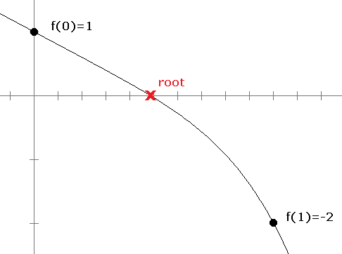

def bisection(f, a, b, n):
    for i in range(n):
        m = (a + b) / 2
        if f(a)*f(m) < 0:
            b = m
        elif f(a)*f(m) > 0:
            a = m
        else:
            return m
    return (a + b) / 2
print(bisection(lambda x:x*x-2, 0, 2, 20))
Analysis of the algorithm
 So in the example above, if we wanted to know how many iterations we would need to get to within ε = 10–6 of the correct answer, we would need ceiling( log2(1/10–6)–1) = 19 iterations.
False position
 This is the point we use in place of the midpoint. Doing so usually leads to faster convergence than the bisection method, though it can sometimes be worse.
Fixed point iteration
from math import cos
x = 2
for i in range(20):
    x = cos(x)
    print(x)
-0.4161468365471424
0.9146533258523714
0.6100652997429745
0.8196106080000903
0.6825058578960018
0.7759946131215992
0.7137247340083882
0.7559287135747029
0.7276347923146813
0.7467496017309728
0.7339005972426008
0.7425675503014618
0.7367348583938166
0.740666263873949
0.7380191411807893
0.7398027782109352
0.7386015286351051
0.7394108086387853
0.7388657151407354
0.7392329180769628
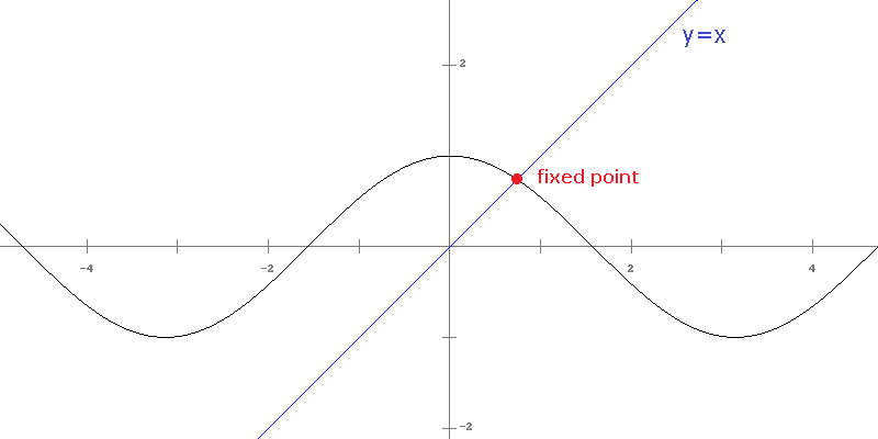
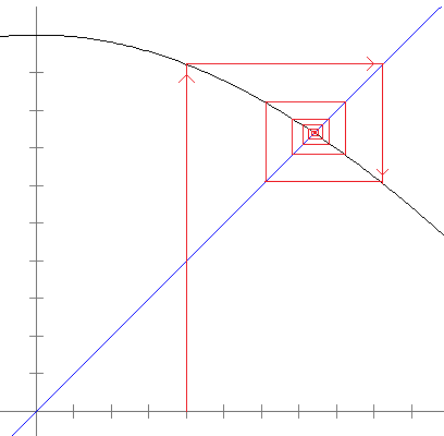
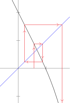
Using fixed points to solve equations
0.484375
0.48666851269081235
0.48634988700459447
0.48639451271206546
0.4863882696148348
0.48638914315650295
0.4863890209322015
0.48638903803364786
0.4863890356408394
0.48638903597563754
0.4863890359287931
0.4863890359353475
0.48638903593443045
0.48638903593455873
0.4863890359345408
0.4863890359345433
0.48638903593454297
0.486389035934543
0.48638903593454297
0.486389035934543
(1-Ans^5)/2 and repeatedly pressing enter. In Excel you can accomplish the same thing by entering .5 in the cell A1, then entering the formula =(1-A1^5)/2 into cell A2, and filling down. Here also is a Python program that will produce the above output:
x = .5
for i in range(20):
    x = (1-x**5)/2
    print(x)
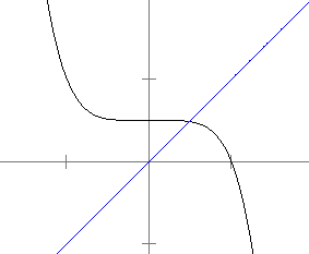
Newton's method
 To see why this is useful, let's look at the derivative of the expression on the left side. We get
 We started with the equation f(x) = 0, so we can plug in 0 for f(x) to turn the above into
 So the derivative at the fixed point is 0. Remember that the flatter the graph is around a fixed point, the faster the convergence, so we should have pretty fast convergence here.
 Then we pick a starting value for the iteration, preferably something we expect to be close to the root of f, like .5. We then iterate the function. Using a calculator, computer program, spreadsheet, or whatever (even by hand), we get the following sequence of iterates:
0.4864864864864865
0.4863890407290883
0.486389035934543
0.486389035934543
0.486389035934543
Ans-(1-2*Ans-Ans^5)/(-2-5*Ans^4) and repeatedly press enter. In Excel, enter .5 in the cell A1, put the formula =A1-(1-2*A1-A1^5)/(-2-5*A1^4) into cell A2, and fill down. Here also is a Python program that will produce the above output, stopping when the iterates are equal to about 15 decimal places:
oldx = 0
x = .5
while abs(x - oldx) > 1e-15:
    oldx, x = x, x-(1-2*x-x**5)/(-2-5*x**4)
    print(x)
Geometric derivation of Newton's method
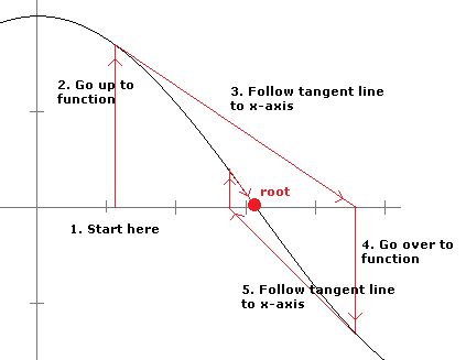
What can go wrong with Newton's method
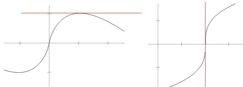
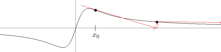
.960, .154, .520, .998, .006, .025, .099, .358, .919, .298, .837, .547,
.991, .035, .135, .466, .995, .018, .071, .263, .774, .699, .842, .532,
.996, .016, .064, .241, .732, .785, .676, .876, .434, .983, .068, .252,
.754, .742, .765, .719, .808, .620, .942, .219, .683, .866, .464, .995
.400     .401
.960     .960
.154     .151
.520     .512
.998     .999
.006     .002
.025     .009
.099     .036
.358     .137
.919     .474

Newton's method and the Babylonian method for roots
 And we see this is actually the Babylonian method formula.
Rates of convergence
xi ei ei+1/ei 0.5000 0.1823 0.645 0.8000 0.1177 0.617 0.6098 0.0726 0.643 0.7290 0.0466 0.629 0.6530 0.0293 0.639 0.7011 0.0187 0.633 0.6705 0.0119 0.637 0.6899 0.0075 0.634 0.6775 0.0048 0.636 0.6854 0.0030 0.635 ei 0.067672196171981 0.003718707799888 0.000011778769295 0.000000000118493 The difference between linear and quadratic convergence
e2 = .01
e3 = .001
e4 = .0001
e5 = .00001
e2 = .01
e3 = .0001
e4 = .00000001
e5 = .0000000000000001
Rates of convergence of bisection, FPI and Newton's method
Generalizations of Newton's method
 Halley's method converges cubically. Halley's method and Newton's method are special cases of a more general class of algorithms called Householder's methods, which have convergence of all orders. However, even though those methods converge very quickly, that fast convergence comes at the cost of a more complex formula, requiring more operations to evaluate. The amount of time to compute each iterate may outweigh the gains from needing less iterations.
The Secant method
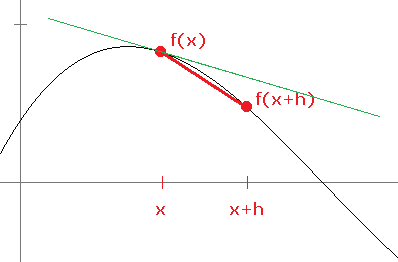
 It is helpful to explicitly describe the iteration as follows:
 That is, the next iterate comes from applying the Newton's method formula to the previous iterate. For the secant method, we replace the derivative with slope of the secant line created from the previous two iterates and get:
 We can then apply a little algebra to simplify the formula into the following:
 Note that this method actually requires us to keep track of two previous iterates.
 We then compute x3 in the same way, using x1 and x2 in place of x0 and x1. Then we compute x4, x5, etc. Here are the first few iterates:
0.9393939393939394
0.6889372446790889
0.5649990748325172
0.49771298490941546
0.48690106666448396
0.4863920162110657
0.4863890367053524
0.48638903593454413
0.486389035934543
0.486389035934543
An implementation in Python
def secant(f, a, b, toler=1e-10):
    while f(b)!=0 and abs(b-a)>toler:
        a, b = b, b - f(b)*(b-a)/(f(b)-f(a))
    return b
secant(lambda x:1-2*x-x**5, 2, 1)
a to the old value of b and b to the value from the secant method formula.
An alternative formula
 where h is a small, but not too small, number (10–5 is a reasonably good choice). The denominator is a numerical approximation to the derivative. However, the secant method is usually preferred to this technique. The numerical derivative suffers from some floating-point problems (see Section 4.1), and this method doesn't converge all that much faster than the secant method.
Muller's method, inverse quadratic interpolation, and Brent's Method
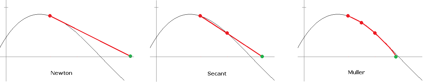
 This comes from finding the equation of the parabola through the three points and solving it using the quadratic formula. The form of the quadratic formula used here is one that suffers less from floating-point problems caused by subtracting nearly equal numbers.

Brent's method
Ridder's method
 The sign of the ± is positive if f(a) > f(b) and negative otherwise. We then adjust a or b just like in the bisection method, setting a = z if f(a) and f(z) have the same sign and b = z otherwise. Repeat the process as many times as needed.
Some more details on root-finding
Speeding up convergence
 This is essentially an algebraic transformation of the original sequence. It comes from fact that once we are close to a root, the ratio of successive errors doesn't change much. That is,

def fpid2(g,s,n):
    x,x1,x2 = s,g(s),g(g(s))
    for i in range(n):
        x,x1,x2 = x1,x2,g(x2)
        print(x,(x2*x-x1*x1)/(x2-2*x1+x))
FPI sped up FPI 0.87758 0.73609 0.63901 0.73765 0.80269 0.73847 0.69478 0.73880 0.76820 0.73896 0.71917 0.73903 0.75236 0.73906 0.73008 0.73907 0.74512 0.73908 0.73501 0.73908 Finding roots of polynomials
 In the denominator, choose whichever sign makes the absolute value of the denominator larger. Keep iterating to find x2, x3, etc. The method converges cubically, so we usually won't need many iterations.
 Then take the derivative of both sides of this expression twice to get


 A little algebra allows us to solve for a to get the formula from the iterative process described above. See A Friendly Introduction to Numerical Analysis by Bradie for a more complete derivation.**Most of the discussion about Laguerre's method here is based off of Bradie's on pages 128-131.
def eval_poly(P, x):
    p, q, r = P[-1], 0, 0

    for c in P[-2::-1]:
        r = r*x + q
        q = q*x + p
        p = p*x + c

    return p, q, 2*r
Finding all the roots of an equation
Most of the methods we have talked about find just one root. If we want to find all the roots of an equation, one option is to find one (approximate) root r, divide the original equation by x–r and then apply the method again to find another. This process is called deflation.
Finding complex roots
Systems of nonlinear equations
Some of the methods, like Newton's method and the secant method, can be generalized to numerically solve systems of nonlinear equations.
Measuring the accuracy of root-finding methods
while abs(x - oldx) > .0000001:
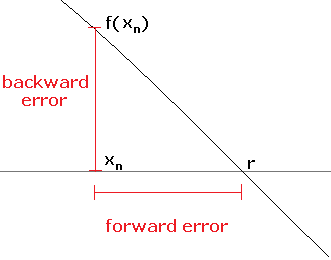
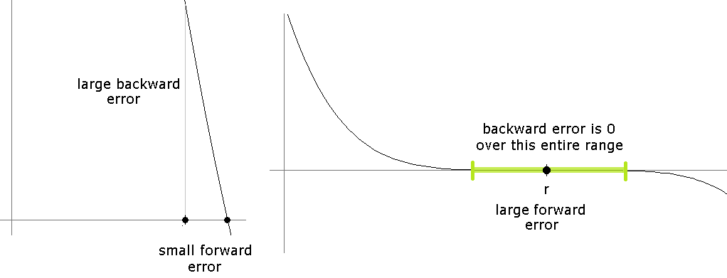
What can go wrong with root-finding
These methods generally don't do well with multiple roots
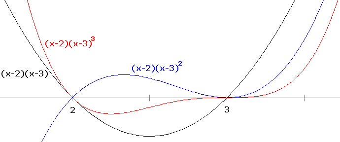
Sensitivity to small changes
The Wilkinson polynomial is the polynomial W(x) = (x–1)(x–2)(x–3) ·s(x–20). In this factored form, we can see that it has simple roots at the integers 1 through 20. Here are a few terms of its expanded form:

Root-finding summary
Interpolation

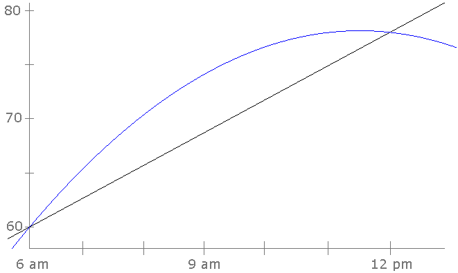
The Lagrange form
 where for each k = 1, 2, … n, we have
 A hat over a term means that that term is not to be included.
 We then plug in the data to get
 Plug these into
 and simplify to get
 We could further simplify this, but sometimes a factored form is preferable.**If we were to simplify it, we would get –35x2+335x+60, which is what we got in the previous section using the system of equations. Lagrange's formula is useful in situations where we need an actual formula for some reason, often in theoretical circumstances. For practical computations, there is a process, called Newton's divided differences, that is less cumbersome to use.**Things like this often happen in math, where there is a simple process to find the answer to something, while an explicit formula is messy. A good example is solving cubic equations. There is a formula akin to the quadratic formula, but it is rather hideous. On the other hand, there is a process of algebraic manipulations that is much easier to use and yields the same solutions.
Newton's divided differences
0 1 2–12–0 = 1/2 2 2 2–1/23–0 = 1/2 4–23–2 = 2 3 4  The coefficients come from the top “row” of the table, the boxed entries. The x terms are progressively built up using the x-values from the first column.
0 2 5–23–0 = 1 3 5 5–14–0 = 1 10–54–3 = 5 –2–16–0 = -1/2 4 10 –1–56–3 = –2 8–106–4 = –1 6 8  One nice thing about this approach is that if we add a new point, we can add it to the bottom of the previous table and not have to recompute the old entries. For example, if we add another point, (5, 8), here is the resulting table:
0 2 5–23–0 = 1 3 5 5–14–0 = 1 10–54–3 = 5 –2–16–0 = –1/2 4 10 –1–56–3 = –2 1––1/27–0 = 3/14 8–106–4 = –1 2––27–3 = 1 6 8 5––17–4 = 2 13–87–6 = 5 7 13 
A general definition
 The notation here differs from the usual way Newton's Divided Differences is defined. The Wikipedia page http://en.wikipedia.org/wiki/Divided_differences has the usual approach.
A practical example
Here is world population data for several years:
Year Millions of people 1960 3040 1970 3707 1990 5282 2000 6080 1960 3040 66.7 1970 3707 .4017 78.75 –.0092 1990 5282 .0350 79.8 2000 6080  Plugging in x = 1980 gives 4473 million people in 1980, which is not too far off from the actual value, 4454. Note that this function interpolates pretty well, but it should not be used for extrapolating to years not between 1960 and 2000. While it does work relatively well for years near this range (e.g., for 2010 it predicts 6810, which is not too far off from the actual value, 6849), it does not work well for years far from the range. For instance, it predicts a population of about 50 billion in 1800. The figure below shows the usable range of the function in green:
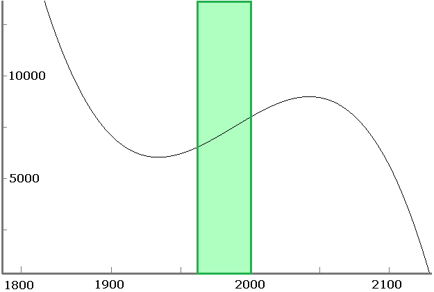
Neville's algorithm
1 11 (2–1) · 15 – (2–3) · 113–1 = 13 3 15 (2–1) · 10 – (2–4) · 134–1 = 12 (2–3) · 20 – (2–4) · 154–3 = 10 (2–1) · 7 – (2–5) · 125–1 = 10.75 4 20 (2–3) · 16 – (2–5) · 105–3 = 7 (2–4) · 22 – (2–5) · 205–4 = 16 5 22 
Problems with interpolation
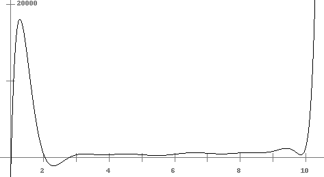
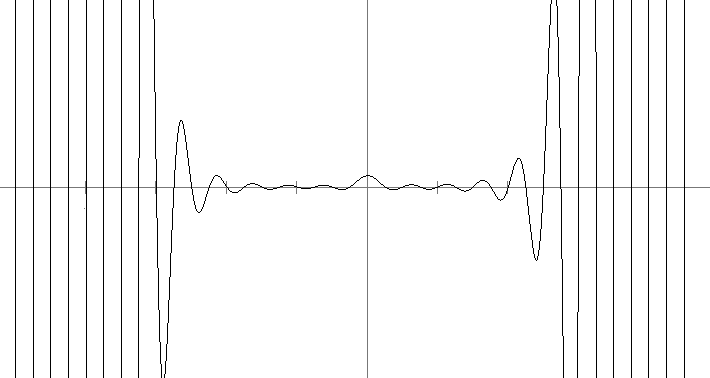
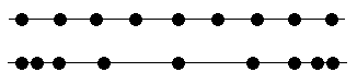


Chebyshev polynomials
 This doesn't look anything like a polynomial, but it really is one. For the first few values of n, we get
 The formula for T2(x) comes from the identity cos(2θ) = 2 cos2θ–1. We can keep going to figure out T3(x), T4(x), etc., but the trig gets messy. Instead, we will make clever use of the trig identities for cos(α ± β). Let y = arccos x. Then we have
 Similarly, we can compute that
 If we add these two equations, we get
 In other words, we have found a recursive formula for the polynomials. Namely,
 Using the fact that T0(x) = 1 and T1(x) = x, we can use this formula to compute the next several polynomials:
 There a few things we can quickly determine about the Chebyshev polynomials:
 For example, if n = 8, the roots are cosπ16, cos3π16, cos5π16, cos7π16, cos9π16, cos11π16, cos13π16, and cos15π16. Note that in the formula above, if i > n, then we would fall outside of the interval [–1, 1].
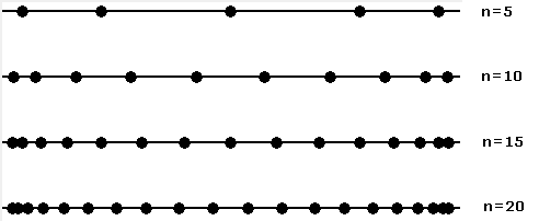
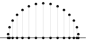

Example
As an example, suppose we want to interpolate a function on the range [0, 20] using 5 points. The formulas above tell us what points to pick in order to minimize interpolation error. In particular,

Error formula
 where the max is taken over the interval [a, b].
A comparison
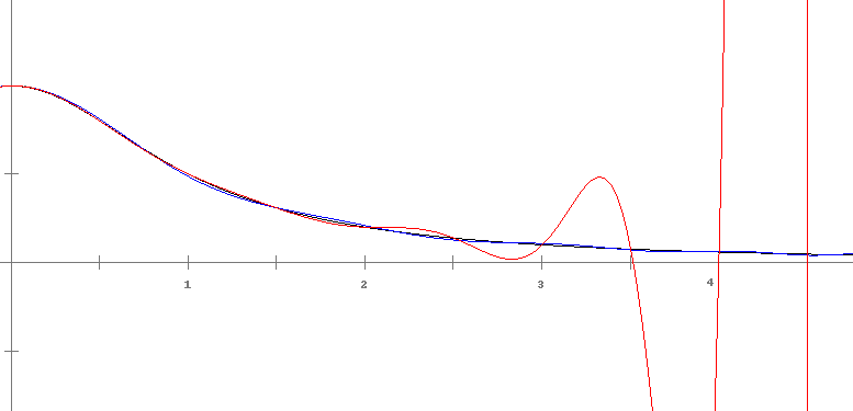
Approximating functions
 Then using Newton's divided differences, we get the following polynomial (with all the coefficients shown to four decimal places for brevity):
 The polynomial and ln x are shown below.
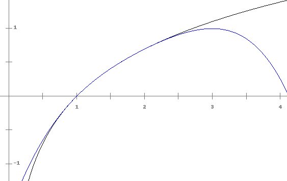
 We can use our polynomial to estimate ln(20/16) and we can compute ln 2 by other means and get an approximate answer that turns out to be off by about 3.3 × 10⁻⁵.
General techniques for approximating functions
 In other words, we can write the sine function as a polynomial, provided we use an infinitely long polynomial. We can get a reasonably good approximation of sin x by using just the few terms from the series. Shown below are a few such approximations.
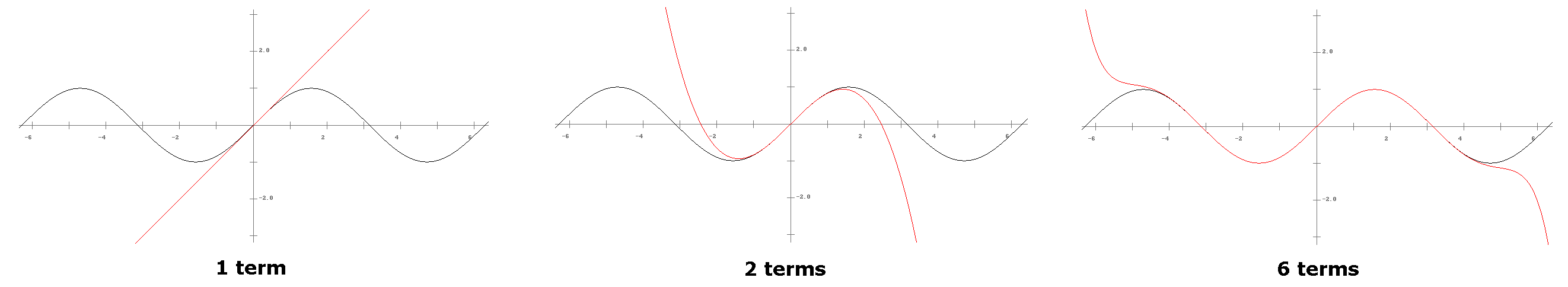
 For example, if we want the Taylor series of f(x) = cos x centered at a = 0, we would start by computing derivatives of cos x. The first few are f′(x) = – sin x, f″(x) = – cos x, f‴(x) = sin x, and f(4)(x) = cos x. Since f(4)(x) = f(x), we will have a nice repeating pattern in the numerator of the Taylor series formula. Plugging a = 0 into each of these and using the Taylor series formula, we get
 Taylor series are often very accurate near the center but inaccurate as you move farther away. This is the case for cos x, but there things we can do to improve this. To start, let's move the center to π/4. An approximation using six terms is
 Its graph is shown below:
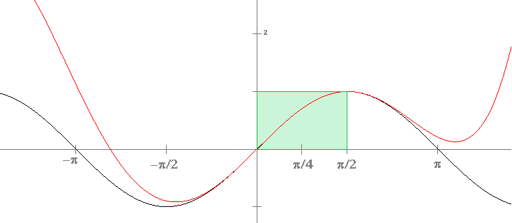
Fourier series
 where we want to find what the coefficients cn are. For Taylor series, those coefficients are determined using derivatives and factorials. We can generalize this idea and try to write f(x) using different types of terms. For example, a very important type of expansion is the Fourier series expansion, where we replace the terms of the form (x–a)n with sines and cosines. Specifically, we try to write
 The goal is to determine c0 and the an and bn. There are simple formulas for them involving integrals that we won't go into here. We can then cut off the series after a few terms to get an approximation to our function. Fourier series are especially useful for approximating periodic functions. Practical applications include signal processing, where we take a complicated signal and approximate it by a few Fourier coefficients, thereby compressing a lot of information into a few coefficients.

 Here are what a few of the approximations look like:
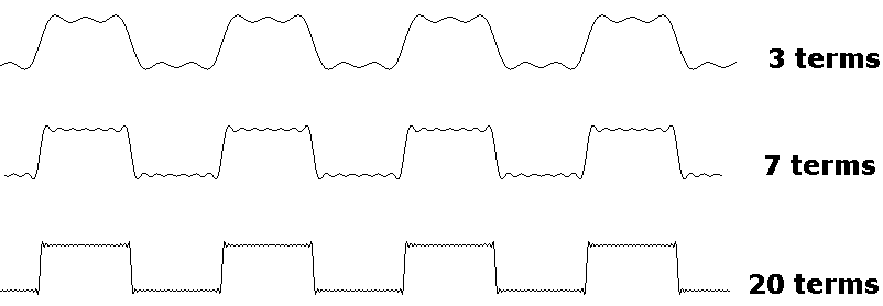
Other types of approximations
 The goal is to find the coefficients cn. This is called Chebyshev approximation.
To approximate f(x) on [a, b] using N terms of the series, set s = (b–a)/2, m = (b+a)/2, and compute
The goal is to find the coefficients cn. This is called Chebyshev approximation.
To approximate f(x) on [a, b] using N terms of the series, set s = (b–a)/2, m = (b+a)/2, and compute
 where
where
 Chebyshev approximation has the property that you don't need very many terms to get a good approximation. See Sections 5.8 – 5.11 of Numerical Recipes for more particulars on this.
The CORDIC algorithm
Piecewise linear interpolation
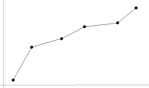
Cubic spline interpolation
 Here is what this might look like:
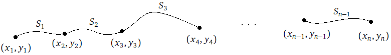
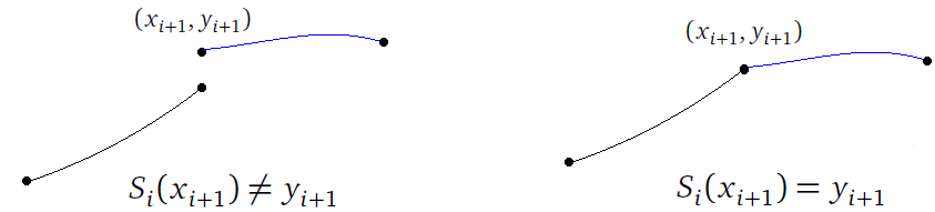
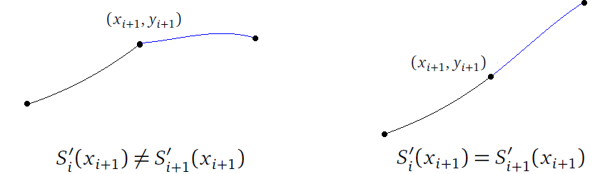


Example:
 This can be solved by row reduction or a more efficient tridiagonal algorithm to get c1 = 0, c2 = 87/64, c3 = –117/32, c4 = 81/64, and c5 = 0. Row reduction can be done using a graphing calculator, various online tools, or a computer algebra system (or by hand if you know the technique and are patient).
Once we have these coefficients, we can plug into the formulas to get
This can be solved by row reduction or a more efficient tridiagonal algorithm to get c1 = 0, c2 = 87/64, c3 = –117/32, c4 = 81/64, and c5 = 0. Row reduction can be done using a graphing calculator, various online tools, or a computer algebra system (or by hand if you know the technique and are patient).
Once we have these coefficients, we can plug into the formulas to get
 This can be done quickly with spreadsheet or a computer program. The equations are thus
 They are graphed below:
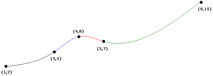
Other types of cubic splines


Interpolation error
Bézier curves
Parametric equations
Many familiar curves are defined by equations like y = x, y = x2, or x2+y2 = 9. But consider the curve below:
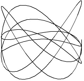
 Thinking of this as the motion of a physical object, t stands for time, and the equations x(t) and y(t) describe the position of the particle in the x and y directions at each instant in time.
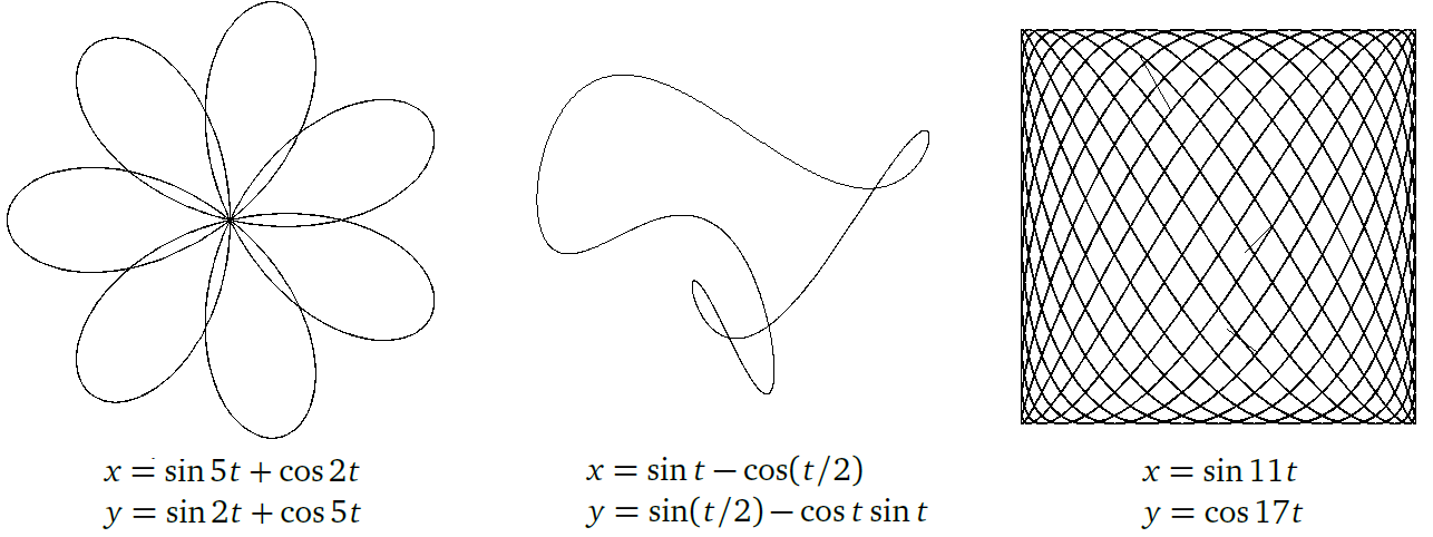
How Bézier curves are defined
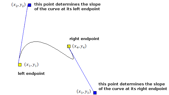
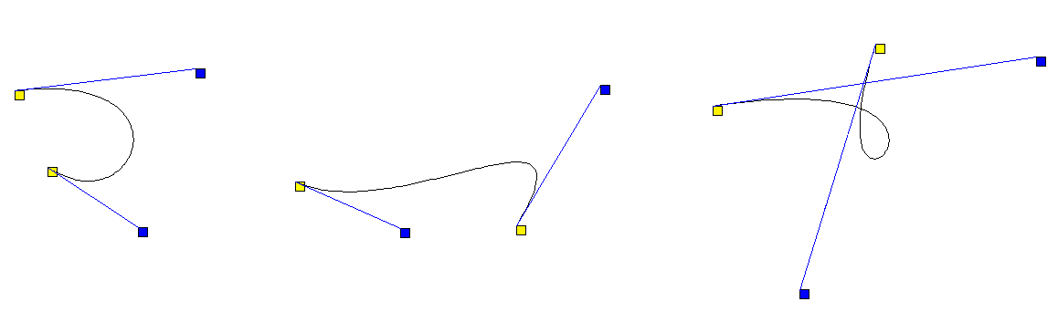

 These equations are valid for 0 ≤ t ≤ 1, where t = 0 gives the left endpoint and t = 1 gives the right.
Quadratic Bézier curves
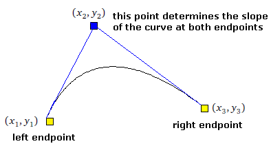

 These equations are valid for 0 ≤ t ≤ 1, where t = 0 gives the left endpoint and t = 1 gives the right.
Summary of interpolation
Further information
Just like with root-finding, we have just scratched the surface here. There are a variety of ways to interpolate that we haven't covered, each with its own pros and cons. For instance, one can interpolate using rational functions (functions of the form p(x)/q(x) where p(x) and q(x) are polynomials). Rational functions are better than polynomials at interpolating functions with singularities.
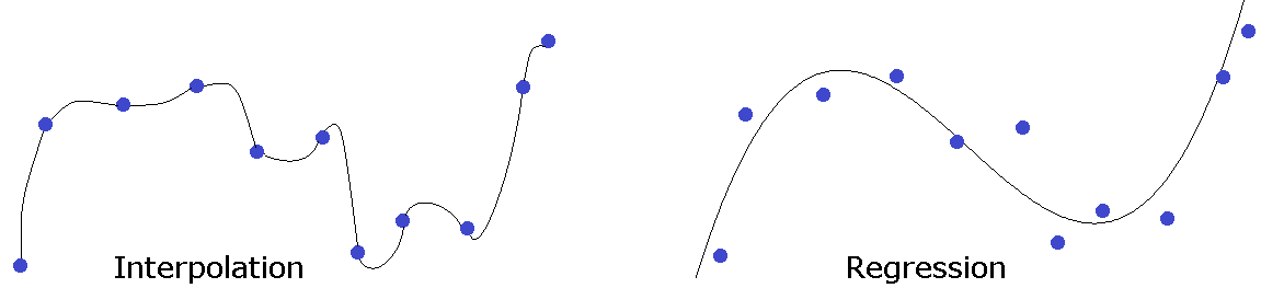
Numerical differentiation
Basics of numerical differentiation
 From this, we see a simple way to estimate the derivative is to pick a small value of h and use it to evaluate the expression inside the limit. For example, suppose we have f(x) = x2 and we want the derivative at x = 3. If we try h = .0001, we get
 This is not too far off from the exact value, 6. The expression, f(x+h)–f(x)h, that we use to approximate the derivative, is called the forward difference formula.
Floating-point error
h (x+h)2–x2h 0.1 6.100000000000012 0.01 6.009999999999849 0.001 6.000999999999479 0.0001 6.000100000012054 10–5 6.000009999951316 10–6 6.000001000927568 10–7 6.000000087880153 10–8 5.999999963535174 10–9 6.000000496442226 10–10 6.000000496442226 10–11 6.000000496442226 10–12 6.000533403494046 10–13 6.004086117172844 10–14 6.217248937900877 10–15 5.329070518200751 Mathematical error
 Replacing x with x+h and taking a = x in the formula above gives the following:
 This is a very useful version of the Taylor series.**It tells us that if we know the value of f(x) and we perturb x by a small amount to x+h, then the function value at that point is f(x)+f′(x)h + f″(x)2!h2+…. Often we approximate the full series by just taking the first couple of terms. For instance, √4 = 2 and if we want √4.1, we could use three terms of the series to estimate it as 2 + 12√4(.1) – 14√4(.1)2 = 2.02374, which is only off by about .001 from the exact value. Using only the first two terms, f(x)+f′(x)h is called a linear approximation and is a common topic in calculus classes.
Solving for f′(x) gives
This is a very useful version of the Taylor series.**It tells us that if we know the value of f(x) and we perturb x by a small amount to x+h, then the function value at that point is f(x)+f′(x)h + f″(x)2!h2+…. Often we approximate the full series by just taking the first couple of terms. For instance, √4 = 2 and if we want √4.1, we could use three terms of the series to estimate it as 2 + 12√4(.1) – 14√4(.1)2 = 2.02374, which is only off by about .001 from the exact value. Using only the first two terms, f(x)+f′(x)h is called a linear approximation and is a common topic in calculus classes.
Solving for f′(x) gives
 All the terms beyond the h2 term are small in comparison to the h2 term, so we might consider dropping them. More formally, Taylor's theorem tells us that
we can actually replace all of the terms from h2 on with f″(c)2!h for some constant c ∈ [x, x+h]. This gives us
All the terms beyond the h2 term are small in comparison to the h2 term, so we might consider dropping them. More formally, Taylor's theorem tells us that
we can actually replace all of the terms from h2 on with f″(c)2!h for some constant c ∈ [x, x+h]. This gives us
 We can read this as saying that f′(x) can be approximated by f(x+h)–f(x)h and the error in that approximation is given by f″(c)2!h. The most important part of the error term is the power of h, which is 1 here. This is called the order of the method.
Combining the two types of errors
Centered difference formula
 Whereas the former approximation looks “forward” from f(x) to f(x+h), the latter approximation is centered around f(x), so it is called the centered difference formula. There is also a backward difference formula, f(x)–f(x–h)h. See the figure below:
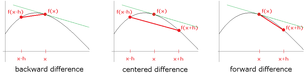
 Subtracting these two equations, dividing by 2h and applying Taylor's formula**There's an additional wrinkle here in that there are actually two different c values from each series, but things do work out so that we only need one value of c in the end. And if you don't want to worry about formalities at all, just imagine that we drop all the terms past the h2 term, since we're only really concerned with the order of the method and not the constants., we see that the f″ term cancels out leaving
 So this is a second order method.
h forward difference centered difference .01 1.0050167084167950 1.0000166667499921 .001 1.0005001667083846 1.0000001666666813 .0001 1.0000500016671410 1.0000000016668897 10–5 1.0000050000069650 1.0000000000121023 10–6 1.0000004999621837 0.9999999999732445 10–7 1.0000000494336803 0.9999999994736442 10–8 0.9999999939225290 0.9999999939225290 10–9 1.0000000827403710 1.0000000272292198 Using Taylor series to develop formulas
 The first part is the numerical differentiation formula that we want and the second part is the error term. We need to find a, b, and c. We start by writing the Taylor expansions for f(x+h) and f(x+2h):
 We want to multiply the first series by b, the second by c, add them together, and solve for f′(x). When we solve for f′(x), we will end up dividing by h. This means that if we want an error term of the form Kh2, it will come from the h3 terms in the Taylor series. Also, since there are no f″ terms in our desired formula, we are going to need those to cancel out when we combine the series. So to cancel out the f″ terms, we will choose b = –4 and c = 1. Then we combine the series to get:
 Note that we could get an expression for K if we want, but since we're mostly concerned with the order, we won't bother.**The actual value of K is 4f‴(c)3! for some c ∈ [x, x+h].. We can then solve this for f′(x) to get
 And to see if our formula works, suppose we try to estimate f′(3) using f(x) = x2 and h = .00001. We get
 which is pretty close to the exact answer, 6.
Higher derivatives
 If we add these two we get
 The key here is that we have canceled out the f′ terms (and as a bonus, the f‴ terms have canceled out as well). Solving for f″(x), we get
 This is a second order approximation for f″.

Note
It is worth noting that all the formulas we've obtained via Taylor series can also be obtained by differentiating the Lagrange interpolating polynomial. For instance, if we write the Lagrange interpolating polynomial through the points (a, f(a)) and (a+h, f(a+h)), and differentiate the result, the forward difference formula results. Further, if we write the interpolating polynomial through (a–h, f(a–h), (a, f(a), and (a+h, f(a+h)), differentiate it, and plug in x = a, then we obtain the centered difference formula. And plugging in x = a–h or x = a+h gives a second-order backward and forward difference formulas.
Richardson extrapolation
 We don't care about the exact values of c1, c2, etc. What we do now is replace h with h/2. We get
 If we multiply the second series by 4 and subtract the first series, we can cancel out the h2 terms. This gives us
 This is now a fourth order method. (Note that we don't care about the exact coefficients of h4, h6, etc., so we just coalesce all of them into Kh4.) We can simplify things down to the following

 This rule has order greater than n.**The term 2nF(h/2)–F(h) is used to cancel out the term of the form Chn in the power series expansion. Note also that one can write Richardson extrapolation in the form Q = 2nF(h)–F(2h)2n–1. For example, let's apply extrapolation to the first-order backward difference formula f(x)–f(x–h)h. We compute
 This method has order 2. This comes from the fact that the power series for the backward difference formula has terms of all orders —c1h+c2h2+c3h3+…—and the extrapolation only knocks out the first term, leaving the h2 and higher terms. On the other hand, sometimes we are lucky, like with the centered difference formula, where the power series has only even terms and we can jump up two orders at once.

 However, as we increase the order, we see that the number of function evaluations increases. This has the effect of slowing down calculation of the numerical derivative. With many numerical methods, there are two competing influences: higher order and number of function evaluations. For numerical differentiation, a higher order means that we don't have to use a very small value of h to get a good approximation (remember that smaller h values cause floating point problems), but we pay for it in terms of the number of function evaluations. The number of function evaluations is a good measure of how long the computation will take. For numerical differentiation, second- or fourth-order methods usually provide a decent tradeoff in terms of accuracy for a given h and the number of required function evaluations.
A tabular approach
Rather than using Richardson extrapolation to create higher order methods, we can apply a tabular approach. We start by using a rule, like the centered difference formula with h values that go down by a factor of 2. So we would use the formula with h = 1, 1/2, 1/4, 1/8, 1/16, …. This gives us a sequence of values that will make up the first column of our table. We'll call them a11, a21, a31, etc.

.708073418273571 .806845360222670 .839769340872369 .832733012957104 .841362230535249 .841468423179441 .839281365458636 .841464149625813 .841470944231850 .841470984248555 .840923259124113 .841470557012606 .841470984171726 .841470984805692 .841470984807877 .841334033327051 .841470958061364 .841470984797948 .841470984807888 .841470984807896 .841470984807896 Automatic differentiation
 All of the higher order terms are 0, since ε2, ε3, etc. are all 0. So the following equation is exact:
 With a little more work, we can show that
 This tells us how to compute function values of dual numbers. For instance,
 Here's where things start to get interesting: Let's look at the product of two functions.
 Look at how the product rule shows up as the component of ε. Next, let's look at the composition of two functions.
 The chain rule somehow shows up as the component of ε. We could similarly show that the quotient rule pops out of dividing two functions.
 This tells us that if we want the (real) derivative of a function, we can subtract f(x+ε)–f(x) and the ε component of that will equal the derivative. The upshot of all this is that we can program all the arithmetical rules for dual numbers as well as the definitions of some common functions, and then our program will almost magically be able to take derivatives of any algebraic combination of those functions, including compositions. Here is a Python implementation of this:
class Dual:
    def __init__(self, a, b):
        self.a = a
        self.b = b

    def __repr__(self):
        return str(self.a)+(" + "+str(self.b) if self.b>=0 else " - "+str(-self.b))+chr(949)

    def __str__(self):
        return self.__repr__()

    def __add__(self, y):
        if type(y) == int or type(y) == float:
            return Dual(self.a + y, self.b)
        else:
            return Dual(y.a+self.a, y.b+self.b)

    def __radd__(self, y):
        return self.__add__(y)

    def __sub__(self, y):
        if type(y) == int or type(y) == float:
            return Dual(self.a-y, self.b)
        else:
            return Dual(self.a-y.a, self.b-y.b)

    def __rsub__(self, y):
        if type(y) == int or type(y) == float:
            return Dual(y-self.a, -self.b)

    def __mul__(self, y):
        if type(y) == int or type(y) == float:
            return Dual(self.a*y, self.b*y)
        else:
            return Dual(y.a*self.a, y.b*self.a + y.a*self.b)

    def __rmul__(self, y):
        return self.__mul__(y)

    def __pow__(self, e):
        return Dual(self.a ** e, self.b*e*self.a ** (e-1))

    def __truediv__(self, y):
        if type(y) == int or type(y) == float:
            return Dual(self.a/y, self.b/y)
        else:
            return Dual(self.a/y.a, (self.b*y.a-self.a*y.b)/(y.a*y.a))

    def __rtruediv__(self, y):
        if type(y) == int or type(y) == float:
            return Dual(y/self.a, -y*self.b/(self.a*self.a))

def create_func(f, deriv):
    return lambda D: Dual(f(D.a), D.b*deriv(D.a)) if type(D)==Dual else f(D)

def autoderiv_nostring(f,x):
    return (f(Dual(x,1))-f(Dual(x,0))).b

def autoderiv(s, x):
    f = eval('lambda x: ' + s.replace("^", "**"))
    return (f(Dual(x,1))-f(Dual(x,0))).b

sin = create_func(math.sin, math.cos)
cos = create_func(math.cos, lambda x:-math.sin(x))
tan = create_func(math.tan, lambda x:1/math.cos(x)/math.cos(x))
sec = create_func(lambda x:1/math.cos(x), lambda x:math.sin(x)/math.cos(x)/math.cos(x))
csc = create_func(lambda x:1/math.sin(x), lambda x:-math.cos(x)/math.sin(x)/math.sin(x))
cot = create_func(lambda x:1/math.tan(x), lambda x:-1/math.sin(x)/math.sin(x))
arcsin = create_func(lambda x:math.asin(x), lambda x:1/math.sqrt(1-x*x))
arccos = create_func(lambda x:math.acos(x), lambda x:-1/math.sqrt(1-x*x))
arctan = create_func(lambda x:math.atan(x), lambda x:1/(1+x*x))
exp = create_func(math.exp, math.exp)
ln = create_func(math.log, lambda x:1/x)
autoderiv("sin(1/x)", 2), the program will automatically differentiate sin(1/x) at x = 2 and give us an answer as accurate as if we were to analytically do the derivative and plug in 2 ourselves.
__add__, __sub__, etc. Then the create_func function is used to build a dual function according to the rule f(a+bε) = f(a) + bf′(a)ε. After that, we use this to program in definitions of common functions like sines and cosines. We do this simply by specifying the function and its derivative. Finally, to compute the derivative, we apply the rule that f′(x)ε = f(x+ε)–f(x), which tells us that the derivative comes from the ε component of f(x+ε)–f(x).
Summary of numerical differentiation
Numerical integration
Newton-Cotes formulas
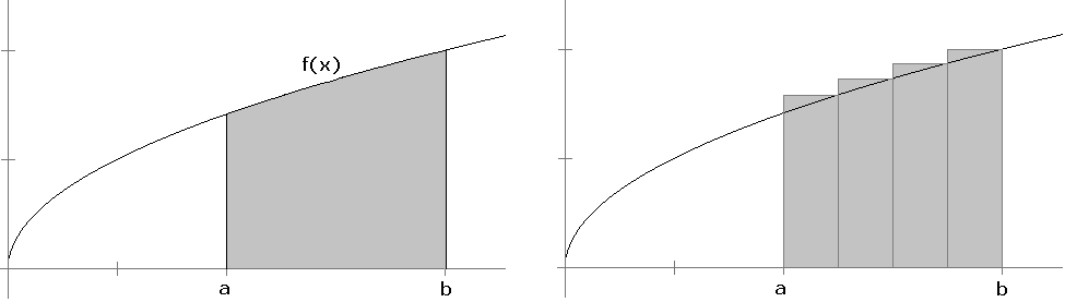
 The exact answer**It is useful to test out numerical methods on easy things so we can compare the estimate with the correct value. is given by 23 x3/2|42 ≈ 3.45. See the figure below.
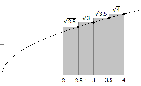
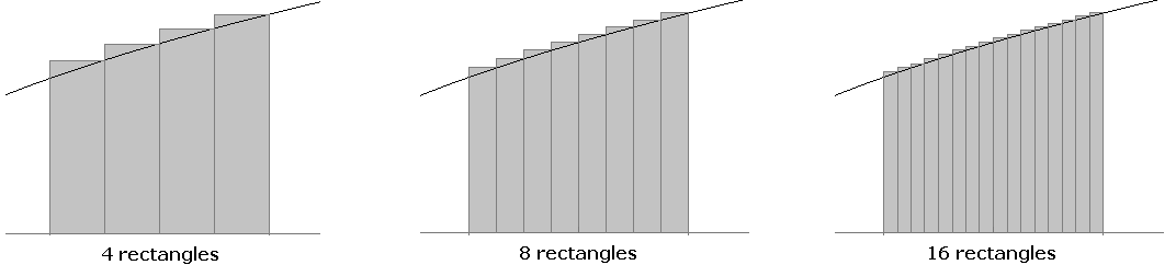
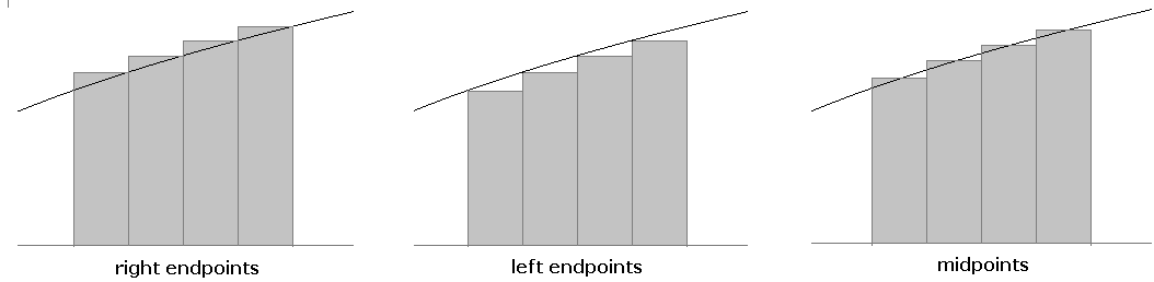
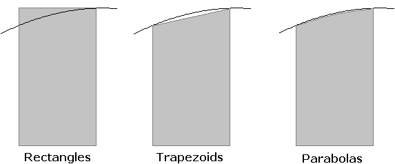
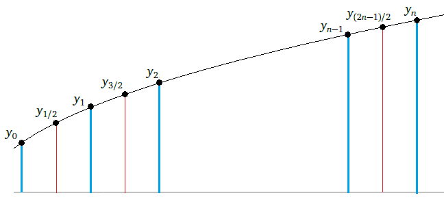
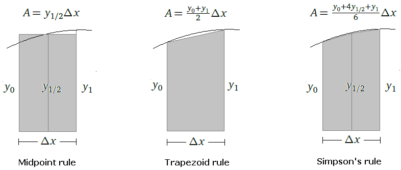


 where S, M, and T denote the Simpson's, midpoint, and trapezoid rules, respectively. This says that Simpson's rule is essentially a weighted average of the midpoint and trapezoid rules.
Example
 The exact answer turns out to be e3–1 ≈ 19.08554. The midpoint estimate is 18.99, the trapezoid estimate is 19.48, and the Simpson's rule estimate is 19.08594, the most accurate of the three by far.
A program
It's pretty quick to write Python programs to implement these rules. For instance, here is the trapezoid rule:
def trapezoid(f, a, b, n):
    dx = (b-a) / n
    return dx/2 * (f(a) + sum(2*f(a+i*dx) for i in range(1,n)) + f(b))
Errors and degree of precision
Rule Error Degree of precision Simple rectangles b–an|max f′| 0 Midpoint rule (b–a)324n2|max f″| 1 Trapezoid rule (b–a)312n2|max f″| 1 Simpson's rule (b–a)52880n4|max f(4)| 3  Solving this, we get n > 1710. So we would need at least 1711 trapezoids to be guaranteed of an error less than .000001, though since the error formula is an overestimate, we could probably get away with fewer.
Higher orders
The iterative trapezoid rule
 Then let's cut the trapezoid exactly in half and use the two resulting trapezoids to estimate the integral:
 The key here is that we already computed part of this formula when we did T1, so we can make use of that. If we cut things in half again, we get
 See the figure below.
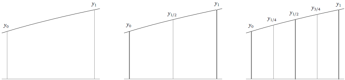
 This method is fairly reliable, even if the function being integrated is not very smooth. In that case, though, it may take a good number of halvings to get to the desired tolerance, leaving an opportunity for roundoff error to creep in. The authors of Numerical Recipes note that this method is usually accurate up to at least 10–10 (using double-precision floating-point).
An example
 Shown below are x-values used at each step:
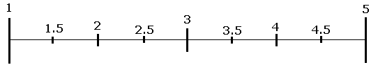
A program
def iterative_trap(f, a, b, toler=1e-10):
    h = b - a
    T = h * (f(a)+f(b))/2
    n = 1
    print(T)
    while n==1 or abs(T - oldT) > toler:
        h = h/2
        n += 1
        T, oldT = T/2 + h * sum(f(a + i*h) for i in range(1, 2**(n-1), 2)), T
        print(T)
Romberg integration
 Applying Richardson extrapolation to the trapezoid rule (which is of order 2), we get for k = 1, 2, …
 We have chosen the symbol S here because extrapolating the trapezoid rule actually gives us Simpson's rule, an order 4 method.
From here, we can extrapolate again to get
We have chosen the symbol S here because extrapolating the trapezoid rule actually gives us Simpson's rule, an order 4 method.
From here, we can extrapolate again to get
 Here, we have chosen the symbol B because extrapolating Simpson's rule gives us Boole's rule, an order 6 method.
T1 T2 S1 T3 S2 B1 … 
 The rest of the entries in the table are then developed from these according to the given extrapolation formulas. One thing to note in the table is that since the order of each extrapolation goes up by 2, the 2n term in the extrapolation formula will become 4n.
Example
Let's try this method on ∫51e–x2 dx. This is the same function we tried with the iterative trapezoid method. The values we found in that example form the first column in Romberg integration. We then use the formulas above to calculate the rest of the values.
.735758882 .368126261 .245582054 .202378882 .147129755 .140566269 .154856674 .139015938 .138475016 .138441822 .143242828 .139371546 .139395253 .139409860 .139413656 .140361311 .139400805 .139402756 .139402875 .139402847 .139402837  If we extend the table by a few more rows, we can get the answer correct to 15 decimal places: 0.1394027926389689. In general, Rn, n will be a much more accurate estimate than Rn, 1, with very little additional computation needed.
Gaussian quadrature
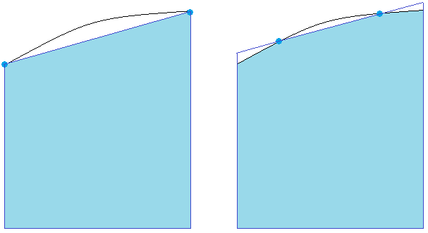
 Plugging in, we get the following two equations:
 We can quickly solve these to get c = –√1/3, d = √1/3. So for any polynomial of degree 2 or less, this rule will exactly integrate it. For example, if f(x) = 4x2+6x–7, we have
 But we also have
 So we have the interesting fact that, we can compute the integral of any quadratic on [–1, 1] just by evaluating it at two points, ±√1/3.

Extending from [–1, 1] to [a, b]
 where p = b–a2 and q = b+a2.
General rule for two-point Gaussian quadrature
To estimate ∫ba f(x) dx, compute p = b–a2, q = b+a2 and then

 To three decimal places, the exact answer is 12.871, so we have done pretty well for just two function evaluations.
A composite method
 The error term for this method (b–a)54320n4|max f(4)|, which is actually a little better than Simpson's rule, and with one less function evaluation.
Gaussian quadrature with more points
 The next two are P2(x) = (3x2–1)/2 and P3(x) = (5x3–3x)/2.

n xi ci 2 –√1/3, √1/3 1, 1 3 –√3/5, 0, √3/5 5/9, 8/9, 5/9 4 -.861136, -.339981, .339981, .861136 .347855, .652145, .652145, .347855  where p = b–a2 and q = b+a2. We could generalize this to a composite rule if we like, but we won't do that here.
 The exact answer is 12.87144 to five decimal places.
A little bit of theory
Adaptive quadrature
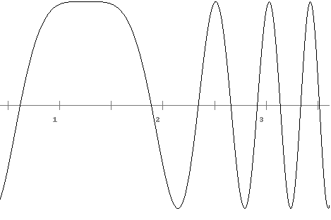
 The terms C1h3, C2(h/2)3, and C3(h/2)3 are the error terms. Each constant is different, but we can make the approximation C1 ≈ C2 ≈ C3 and replace all three with some constant C. Then the difference that we compute in the method is
 That is, the difference is about three times the error of T[a, m]+T[m, b], which is our approximation to ∫ba f(x) dx, so that's where the 3ε comes from.
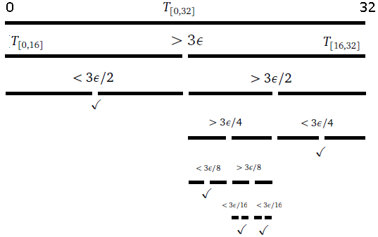
A program
def adaptive_quad(f, a, b, toler):
    m = (a+b) / 2
    T1 = (b-a) * (f(a) + f(b)) / 2
    T2 = (b-a) * (f(a) + f(m)) / 4
    T3 = (b-a) * (f(m) + f(b)) / 4

    if abs(T1-T2-T3)< 3*toler:
        return T2+T3
    else:
        return adaptive_quad(f, a, m, toler/2) + adaptive_quad(f, m, b, toler/2)
T1 and T2 and then it may be computed again in the first recursive call to adaptive_quad. We can speed things up by saving the values of the function evaluations (which can often be slow if the function is complicated) and passing them around as parameters. In addition, the values of T2 and T3 are recomputed as T1 in the recursive calls. If we save these as parameters, we can get a further speed-up. The improved code is below:
def adaptive_quad(f, a, b, toler):
    return adaptive_quad_helper(f, a, b, f(a), f(b), (b-a)*(f(a)+f(b))/2, toler)

def adaptive_quad_helper(f, a, b, fa, fb, T1, toler):
    m = (a+b) / 2
    fm = f(m)
    T2 = (b-a) * (fa + fm) / 4
    T3 = (b-a) * (fm + fb) / 4

    if abs(T1-T2-T3)< 3*toler:
        return T2+T3
    else:
        return adaptive_quad_helper(f, a, m, fa, fm, T2, toler/2) +\
               adaptive_quad_helper(f, m, b, fm, fb, T3, toler/2)
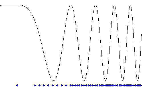
Improper and multidimensional integrals

Integrals with an infinite range of integration
 This gives
 Shown below are the two functions. The shaded areas have the same value.
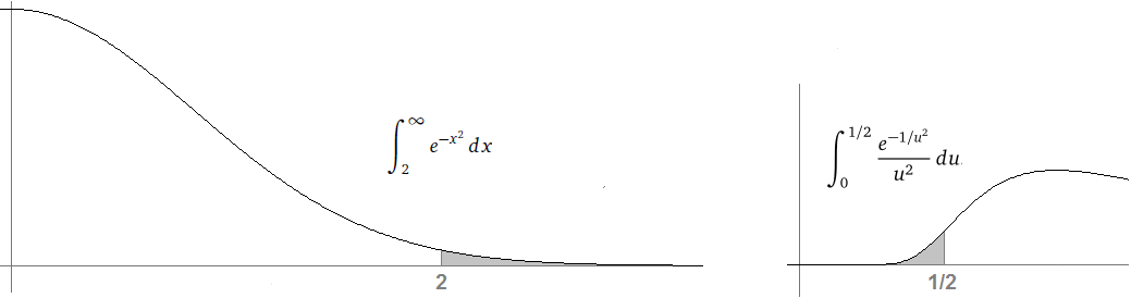

Integrals with discontinuities
 If we don't know where a discontinuity happens, then there are things one can do, but we won't cover them here.
Multiple integrals
Multidimensional integrals are somewhat tougher to handle than single integrals. In general, we have an integral of the form
 where D is some region. If D is not too complicated and f is relatively smooth, then the integral can be evaluated higher-dimensional analogs of some of the methods we talked about, like Gaussian quadrature.
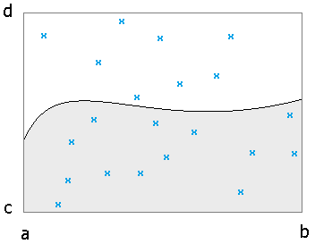
from random import uniform

def monte_carlo_integrate(f, a, b, c, d, num_points):
    inside_count = 0
    for i in range(num_points):
        x = uniform(a,b)
        y = uniform(c,d)
        if y <= f(x):
            inside_count += 1
    return inside_count/num_points * (b-a)*(d-c)
if 0 <= y <= f(x):
    inside_count += 1
else if f(x) <= y <= 0:
    inside_count -= 1
Summary of integration techniques
The preceding sections are not a how-to guide for what algorithms to use when, nor are they are a rigorous development of methods and error bounds.They are just meant to be an overview of some of the methods and key ideas behind numerical integration. For practical information, see Numerical Recipes, and for rigorous derivations, see a numerical analysis textbook.
Numerical methods for differential equations
Initial value problems

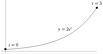
Euler's method
 The equation y′ = ty2+t can be thought of as giving a slope at each point (t, y). If we plot the slopes at every point, we have a slope field, like the one shown below:
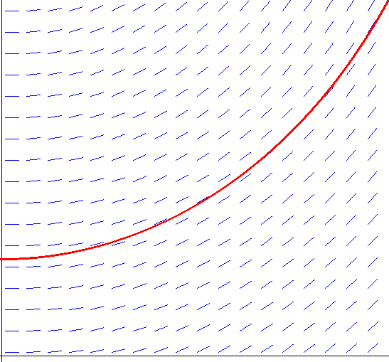
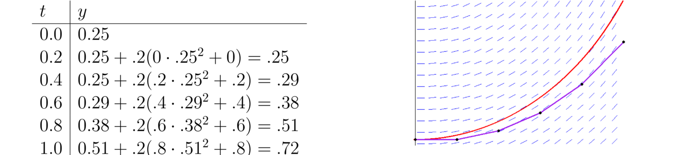

 The step size determines how much we move in the t-direction. The change in the y-direction comes from following the slope for h units from the previous point. That slope is given by plugging in the previous point into the differential equation. We continue generating points until we reach the end of the interval.
A short program
Here is a short Python program implementing Euler's method. The method collects all of the points (t0, y0), (t1, y1), etc. into a list.
def euler(f, y_start, t_start, t_end, h):
    t, y = t_start, y_start
    ans = [(t, y)]
    while t < t_end:
        y += h * f(t,y)
        t += h
        ans.append((t,y))
    return ans
L = euler(lambda t,y: t*y*y+t, .0001, 0, 1, .25)
This stores a rather long list of values in L. If we just want the last tuple (tn, yn), it is in L[-1].We would use L[-1][1] to get just the final y value.**Note that for simplicity, the condition on our while loop is while t < t_end. However, because of roundoff error, we could end up looping too long. For instance, if our interval is [0, 1] and h = .1, then because of roundoff error, our last step will take us to .9999…, which will come out less than 1 and we will end up computing one step too many. We can fix this problem by either asking the caller for the number of steps they want to compute instead of h or by computing it ourselves as n=int(round((t_end-t_start)/h)) and replacing the while loop with for i in range(len(n)).
Problems with Euler's method
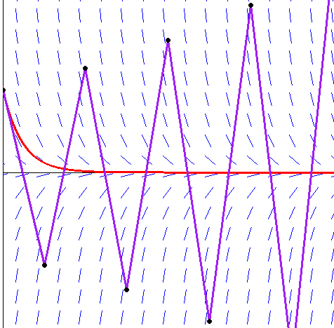
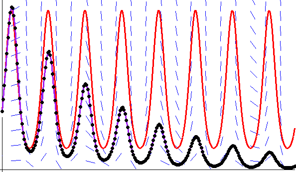
Error in Euler's method
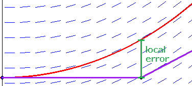
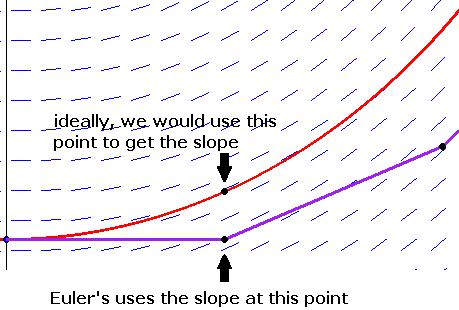
 But y~(t0), the initial condition, is exactly equal to y0, and y~′(t0) is exactly equal to f(y0, t0). So from this we get
 So the local error is on the order of h2.
 where C and L are constants.**L is called a Lipschitz constant. It satisfies |f(t, u)–f(t, v)| ≤ L|u–v| for all points (t, u) and (t, v) in the domain. We notice, in particular, the exponential term, which indicates that the error can eventually grow quite large.
Explicit trapezoid method
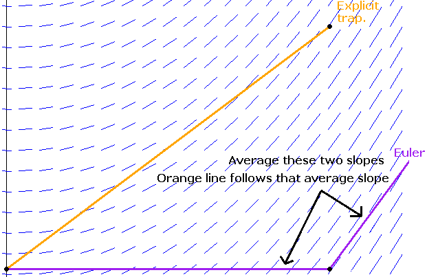

 In the formulas above, s1 is the slope that Euler's method uses, (tn, yn+hs1) is the point that Euler's method wants to take us to, and s2 is the slope at that point. We get yn+1 by following the average of the slopes s1 and s2 for h units from yn.
def explicit_trap(f, y_start, t_start, t_end, h):
    t, y = t_start, y_start
    ans = [(t, y)]
    while t < t_end:
        s1 = f(t, y)
        s2 = f(t+h, y+h*s1)
        y += h*(s1+s2)/2
        t += h
        ans.append((t,y))
    return ans
Example
tn s1 Euler's prediction s2 yn 0 — — — .25 .2 f(0, 1) = 0 .25+(.2)(0) = .25 f(.2, .25) = .21 .25 + .20+.212 = .27 .4 f(.2, .27) = .21 .27+(.2)(.21) = .31 f(.4, .31) = .44 .27 + .2.21+.442 = .34 .6 f(.4, .34) = .45 .34+(.2)(.45) = .43 f(.6, .43) = .71 .34 + .2.45+.712 = .45 .8 f(.6, .45) = .72 .45+(.2)(.72) = .60 f(.8, .60) = 1.08 .45 + .2.72+.1.082 = .63 1 f(.8, .63) = 1.12 .63+(.2)(1.12) = .86 f(1, .86) = 1.73 .63 + .21.12+1.732 = .92 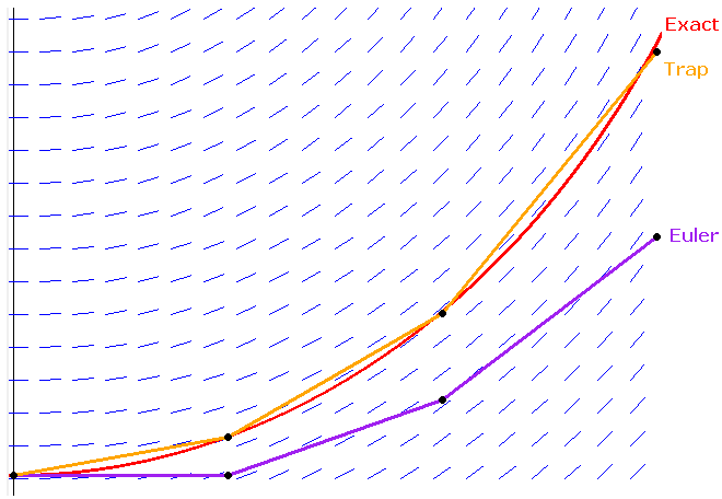
 This is exactly equivalent to the summing of areas of trapezoids, which is what the trapezoid rule for integration does. The result of running the method is essentially a table of approximate values of the antiderivative of f at the values t0, t0+h, t0+2h, etc. achieved from running the trapezoid rule, stopping at each of those points.
The midpoint method
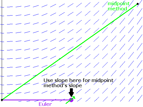

 In the formulas above, s1 is the slope that Euler's method wants us to follow. We do temporarily follow that slope for h/2 units and compute the slope at that point, which we call s2. Then we start back at (tn, yn) and slope s2 for h units to get our new point (tn+1, yn+1). Note that we could also write yn+1 more compactly as follows

Example
Suppose we have the IVP y′ = ty2+t, y(0) = .25, t ∈ [0, 1].
Here are the calculations for the midpoint method using h = .2 (all rounded to two decimal places):
tn s1 y+h2s1 s2 yn 0 — — — .25 .2 f(0, .25) = 0 .25 + (.1)(0) = .25 f(.1, .25) = .11 .25 + (.2)(.10) = .27 .4 f(.2, .27) = .21 .27 + (.1)(.21) = .29 f(.3, .29) = .33 .27 + (.2)(.33) = .34 .6 f(.4, .34) = .45 .34 + (.1)(.45) = .38 f(.5, .38) = .57 .34 + (.2)(.57) = .45 .8 f(.6, .45) = .72 .45 + (.1)(.72) = .52 f(.7, .52) = .89 .45 + (.2)(.89) = .63 1.0 f(.8, .63) = 1.12 .63 + (.1)(1.12) = .74 f(.9, .74) = 1.39 .63 + (.2)(1.39) = .91 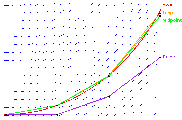
Runge-Kutta methods
 Geometrically, these methods can be described as following the Euler's method prediction α percent of the way from tn to tn+1, computing the slope there, taking a weighted average of that slope and the slope at (tn, yn), and following that average slope from (tn, yn) for h units. See the figure below:
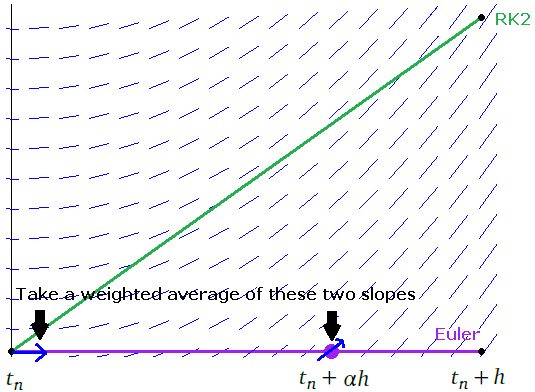

RK4

 The RK4 method builds off of the RK2 methods (trapezoid, midpoint, etc.) by using four slopes instead of two.
The new yn+1 is computed as a weighted average those four slopes. See the figure below:
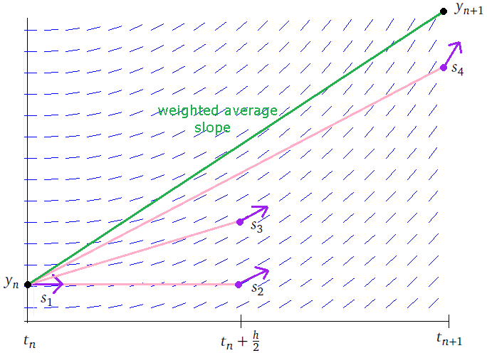
def rk4(f, y_start, t_start, t_end, h):
    t, y = t_start, y_start
    ans = [(t, y)]
    while t < t_end:
        s1 = f(t, y)
        s2 = f(t+h/2, y+h/2*s1)
        s3 = f(t+h/2, y+h/2*s2)
        s4 = f(t+h, y+h*s3)
        y += h * (s1+2*s2+2*s3+s4)/6
        t += h
        ans.append((t,y))
    return ans
Systems of ODEs
 Just to see how things work, let's numerically solve it using Euler's method with h = .5:
tn xn yn 0.0 1 6 0.5 1 + .5(2–(1)(6)+62) = 17 6+.5(3–(1)(6)+12) = 5 1.0 17 + .5(2–(17)(5)+52) = –12 5+.5(3–(17)(5)+172) = 108.5
def euler_system(F, Y_start, t_start, t_end, h):
   t, Y = t_start, Y_start
   ans = [(t_start, Y)]
   while t < t_end:
       Y = [y+h*f(t,*Y) for y, f in zip(Y,F)]
       t+=h
       ans.append((t,Y))
   return ans
L = system([lambda t,x,y: 2-x*y+y*y, lambda t,x,y:3-x*y+x*x], [1,6], 0, 1, .5))

x y s1 = (0 · 3 + 42) = 16 r1 = (3 · 4) = 12 s2 = f(.5, 3+16 ·.5, 4+12 ·.5) = .5 · 11 + 102 = 105.5 r2 = g(.5, 3+16 · .5, 4+12 · .5) = 11 · 10 = 110 x1 = 3 + 105.5 · 1 = 108.5 y1 = 4 + 110 · 1 = 114
def system_mid(F, Y_start, t_start, t_end, h):
    t, Y = t_start, Y_start
    ans = [(t_start, Y)]
    while t < t_end:
        S1 = [f(t, *Y) for f in F]
        Z = [y+h/2*s1 for y,s1 in zip(Y,S1)]
        S2 = [f(t+h/2, *Z) for f in F]
        Y = [y+h*s2 for y,s2 in zip(Y,S2)]
        t+=h
        ans.append((t,Y))
    return ans
Higher order equations
Higher order equations are handled by converting them to a system of first-order equations. For instance, suppose we have the system y″ = y+t. Let's introduce a variable v = y′. We can write the ODE as the system y′ = v, v′ = y+t. We can then use the methods from the previous section to estimate a solution. Note that since our system is second-order, we will have two initial conditions, one for y and one for y′.
tn y v a 0.0 1 3 6 2.0 1 + 2(3) = 7 3 + 2(6) = 15 6 + 2((3)(6)+(4)(1)–02) = 46 4.0 7 + 2(15) = 37 15+ 2(46) = 107 46 + 2((3)(46) + (4)(7) – 22) = 368 Simulating physical systems
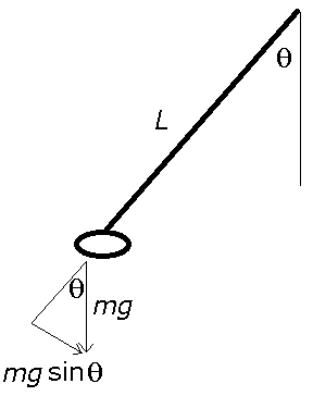
 This equation cannot easily be solved by standard analytic means. We can make it even harder to analytically solve by adding a bit of friction to the system as follows:
 where c is some constant. Despite the difficulty we have in solving it analytically, we can easily find an approximate solution. Here is a Python program that uses Euler's method to numerically estimate a solution and sketches the resulting motion of the pendulum:
from math import sin, cos
from tkinter import *

def plot():
    y = 3
    v = 1
    h = .0005
    while True:
        v, y = v + h*f(y,v), y + h*v
        a = 100*sin(y)
        b = 100*cos(y)
        canvas.coords(line, 200, 200, 200+a, 200+b)
        canvas.coords(bob, 200+a-10, 200+b-10, 200+a+10, 200+b+10)
        canvas.update()

f = lambda y, v: -9.8/1*sin(y)-v/10
root = Tk()
canvas = Canvas(width=400, height=400, bg='white')
canvas.grid()
line = canvas.create_line(0, 0, 0, 0, fill='black')
bob = canvas.create_oval(0, 0, 0, 0, fill='black')
plot()
This program is very minimalistic, with absolutely no bells and whistles, but it fairly accurately simulates the motion of a pendulum. One improvement would be to only plot the pendulum when it has moved a noticeable amount, such as when a or b changes by at least one pixel. This would give a considerable speedup. We could also allow the user to change some of the constants, like the length of the pendulum or the damping factor. And a more accurate result can be obtained by using the RK4 method. We can do this by replacing the first line of the while loop with the following code:
s1 = v
t1 = f(y,v)

s2 = v+h/2*s1
t2 = f(y+h/2*s1, v+h/2*t1)

s3 = v+h/2*s2
t3 = f(y+h/2*s2, v+h/2*t2)

s4 = v+h*s3
t4 = f(y+h*s3, v+h*t3)

v = v + h*(t1+2*t2+2*t3+t4)/6
y = y + h*(s1+2*s2+2*s3+s4)/6
Multistep methods
 The method uses a kind of weighted average of the slopes at (tn, yn) and (tn–1, yn–1). Average isn't really the best term to use here. It's more like we are primarily relying on the slope at (tn, yn) and correcting it slightly with the slope at (tn–1, yn–1).**We could use other weightings, like 5s2–2s13 or 3s2+s14, but the Adams-Bashforth method's weightings have been chosen to give the best possible error term using the two slopes.
def AB2(f, y_start, t_start, t_end, h):
    t, y = t_start, y_start
    s2 = f(t, y)
    y += h*f(t+h/2, y+h/2*f(t,y))  # midpoint method for y_1
    t += h
    ans = [(t_start,y_start), (t,y)]

    while t < t_end:
        s1 = s2
        s2 = f(t, y)
        y += h * (3*s2-s1)/2
        t += h
        ans.append((t,y))
    return ans
 We have used the shorthand fi = f(ti, yi). Note that only one new function evaluation is required at each step.
Implicit methods and stiff equations
 Suppose instead we use the backward difference formula y′(t) = y(t)–y(t–h)h. Solve it to get y(t) = y(t–h) + hy′(t) and take t = tn+1. This leads to the following method:
 This is called the backward Euler method, and it might seem a little bizarre. We are using the slope at very point that we are trying to find, even though we haven't found that point yet. A better way to look at this is that it gives us an equation that we can solve for yn+1. Chances are that the equation will be difficult to solve numerically, so a numerical root-finding method would be necessary. For instance, if we have f(t, y) = (t+1)ey, y(0) = 3, and h = .1, to get y1 we would have to solve the equation y1 = 3 + .1(0+1)ey1, something we can't solve algebraically.
def backward_euler(f, y_start, t_start, t_end, h):
    t, y = t_start, y_start
    ans = [(t, y)]
    while t < t_end:
        g = lambda x:y + h*f(t+h,x)-x
        a, b = y,  y + h*f(t+h/2, y+h/2*f(t,y))
        while g(a)!=g(b) and abs(b-a)>.00000001:
            a, b = b, b - g(b)*(b-a)/(g(b)-g(a))
        y = b
        t += h
        ans.append((t, y))
    return ans
The bulk of the while loop is spent numerically solving for yn+1. We start by setting g equal to the function we need to solve for yn+1, with x standing for yn+1. Our two initial guesses to get the secant method started are y0 and the midpoint method's guess for y1. After the inner while loop finishes, b holds the secant method's estimate for yn+1.

 using the trapezoid rule for integration gives the implicit trapezoid method. If we use Simpson's rule to do the integration, we get yn+1 = yn + fn+1+4fn+fn–13, a fourth-order method called the Milne-Simpson method. There are also some useful implicit methods in the Runge-Kutta family, though we won't cover them here.
Stiff equations
 Its exact solution is y = e–4.25t. Shown below is the result of applying Euler's method with a step size of h = .5:
Predictor-corrector methods
 We then find yn+1 with a root-finding method. Here is a different approach: Suppose we use the regular Euler method to generate an approximate value for yn+1 and use that in the backwards Euler formula. We would have the following method (where y~n+1 represents the Euler's method prediction):
 The idea is that Euler's method predicts yn+1 and the backward Euler method corrects the prediction. This is a simple example of a predictor-corrector method. Predictor-corrector methods are explicit methods. Note the similarity of this method to the explicit trapezoid rule.
 We have used the shorthand fi = f(ti, yi). Here is the combined method:
 Here f~n+1 = f(tn+1, y~n+1). This method requires four values to get started. The first is the initial value, and the next three can be generated by RK4 or another explicit method.
Variable step-size methods
def simple_adaptive(f, y_start, t_start, t_end, h, T=.0001):
    t, y = t_start, y_start
    ans = [(t, y)]

    while t < t_end:
        s1 = f(t, y)
        s2 = f(t+h/2, y+h/2*s1)

        euler = y + s1*h
        midpt = y + s2*h
        e = abs(midpt-euler)

        # estimate is no good, decrease step size and try this step over
        if e > T:
            h /= 2

        # estimate is very good, increase step size
        elif e < T/10:
            y = midpt
            t += h
            ans.append((t,y))
            h *= 2

        # estimate is acceptable, keep same step size for next step
        else:
            y = midpt
            t += h
            ans.append((t,y))

    return ans
 The fourth-order approximation is wn and the fifth-order approximation is zn. Our error estimate is
 We divide by h here to get the relative error.
 This scaling factor can be shown analytically to be a good choice. In practice, if Δ < .1, we set Δ = .1 and if Δ > 4, we set Δ = 4, both in order to avoid too drastic of a change in step size. Also in practice, the user is allowed to specify a minimum and maximum value for h.
def rkf45(f, y_start, t_start, t_end, h, T=.0001, max_h=1):
    t, y = t_start, y_start
    ans = [(t, y)]

    while t < t_end:
        s1 = h*f(t, y)
        s2 = h*f(t+(1/4)*h, y+(1/4)*s1)
        s3 = h*f(t+(3/8)*h, y+(3/32)*s1+(9/32)*s2)
        s4 = h*f(t+(12/13)*h, y+(1932/2197)*s1-(7200/2197)*s2+(7296/2197)*s3)
        s5 = h*f(t+h, y+(439/216)*s1-8*s2+(3680/513)*s3-(845/4104)*s4)
        s6 = h*f(t+(1/2)*h, y-(8/27)*s1+2*s2-(3544/2565)*s2+(1859/4104)*s4-(11/40)*s5)

        w = (25/216)*s1 + (1408/2565)*s3 + (2197/4104)*s4 - (1/5)*s5
        e = abs((1/360)*s1 - (128/4275)*s3 - (2197/75240)*s4 + (1/50)*s5 + (2/55)*s6)/h

        delta = .84 * abs(T/w)**.2
        delta = min(delta, 4)
        delta = max(delta, .1)

        # estimate is very good, increase step size
        if e < T/10:
            y += (16/135)*s1 + (6656/12825)*s3 + (28561/56430)*s4 - (9/50)*s5 + (2/55)*s6
            t += h
            h = min(h / delta, max_h)
            ans.append((t,y))

        # estimate is no good, decrease step size and try this step over
        elif e > T:
            h = h * delta
            if h < min_h:
                raise Exception("Forced to use step size less than minimum")

        # estimate is acceptable, keep same step size for next step
        else:
            y += (16/135)*s1 + (6656/12825)*s3 + (28561/56430)*s4 - (9/50)*s5 + (2/55)*s6
            t += h
            ans.append((t,y))

    return ans
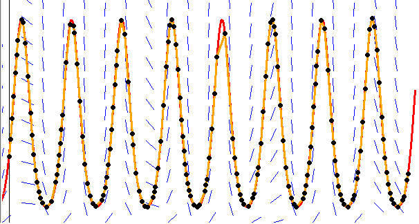
Extrapolation methods
 We see why it is called the leapfrog method: we leap from yn–1 to yn+1, jumping over yn (though using the slope there). We can also see that it is closely related to the midpoint method. A benefit of this method over the usual midpoint method is that this method requires only one new function evaluation at each step, as opposed to the two that the midpoint method requires.

A little about why extrapolation works
 where the series includes only even terms. If we use a step size of h to get R11 and a step size of h/2 to get R21, then when we compute
R22 = 4R21–R113, the h2 terms cancel out:
where the series includes only even terms. If we use a step size of h to get R11 and a step size of h/2 to get R21, then when we compute
R22 = 4R21–R113, the h2 terms cancel out:
 This means that R22 is a fourth order approximation.
When we compute R33 = 16R22–R3215, the h4 terms cancel out, leaving a 6th order approximation. In general, the order goes up by 2 with each successive level of extrapolation.
This means that R22 is a fourth order approximation.
When we compute R33 = 16R22–R3215, the h4 terms cancel out, leaving a 6th order approximation. In general, the order goes up by 2 with each successive level of extrapolation.
 The denominator is not necessary to zero out the h2 term, but it is needed to keep everything scaled properly. The entire expression acts as a sort of odd weighted average with negative weights.
 This is precisely the formula used by Neville's formula for polynomial interpolation, evaluated at h = 0. You may recall that Neville's formula is a close relative of Newton's divided differences. And, indeed, when we do this extrapolation process, we make a table that is reminiscent of the ones we make when doing polynomial interpolation. This because this extrapolation process is really the same thing. We are trying to fit a polynomial to our data and extrapolate to get an estimate of the value at a step size of h = 0.
 If we put these values into a table and run extrapolation, here is what we get:
1/2 3.149041 1/4 3.144575 3.143087 1/6 3.143303 3.142285 3.142185 1/8 3.142737 3.142010 3.141918 3.141900 1/10 3.142428 3.141879 3.141805 3.141783 3.141778 1/12 3.142237 3.141804 3.141745 3.141725 3.141717 3.141716 1/14 3.142110 3.141757 3.141708 3.141691 3.141683 3.141680 3.141679 1/16 3.142020 3.141725 3.141684 3.141669 3.141662 3.141659 3.141657 3.141657 Code for the extrapolation algorithm
def neville(X, Y):
    R = [Y]
    for i in range(1,len(Y)):
        L = []
        for j in range(1,len(R[i-1])):
            L.append((X[i+j-1]**2*R[i-1][j]-X[j-1]**2*R[i-1][j-1])/(X[i+j-1]**2-X[j-1]**2))
        R.append(L)
    return R
def extrapolate(f, y_start, t_start, t_end, H):
    ans = [(t_start, y_start)]
    start = t_start
    end = t_start + H
    while end < t_end:
        h = end - start
        n = 8
        X = []
        Y = []

        for i in range(n):
            h  = (end-start)/(2*(i+1))
            t, y, oldy = start, y_start, y_start
            y += h*f(t+h/2, y+h/2*f(t,y))
            t += h
            for j in range(2*(i+1)):
                oldy, oldy2 = y, oldy
                y = oldy2 + 2*h*f(t, y)
                t += h
            X.append(2*(i+1))
            Y.append(oldy)

        N = neville(X,Y)
        ans.append((end, N[n-1][0]))
        start, end = end, end + H
        y_start = N[n-1][0]
    return ans
Summary and Other Topics
Exercises
Exercises for Chapter 1
(a) exactly .3
(b) a number within around 4 × 10–17 of .3
float and double data types of many programming languages?
    if price1 + price2 == 89.9:
        print("Everything's free!!!")
Exercises for Chapter 2


f = lambda x:x**10-11*x**9+54*x**8-156*x**7+294*x**6-378*x**5+336*x**4
-204*x**3+81*x**2-19*x+2

df = lambda x:10*x**9-99*x**8+432*x**7-1092*x**6+1764*x**5-1890*x**4
+1344*x**3-612*x**2+162*x-19


A61. Column C contains the error ratios ei+1/ei. Recreate this spreadsheet. An example of the first few lines is shown below.

if() expressions in Excel and also how to use the MOD() function.

Decimal class, the Java BigDecimal class, or another programming language's decimal class to estimate the solution of 1–2x–x5 = 0 correct to 50 decimal places.
my_sqrt that computes √n as accurately as the programming language's own sqrt function (but without using the language's sqrt or power functions).
Exercises for Chapter 3
year percent 1986 16.3% 1992 18.4% 1998 22.5% 2008 29.8% 2014 35.1%
(1) L(x) and p(x) are actually always the same
(2) L(x) and p(x) usually agree except for a few very unusual examples
(3) L(x) and p(x) most of the time are different.
cheb(5) should return 16x^5-20x^3+5x.
Exercises for Chapter 4
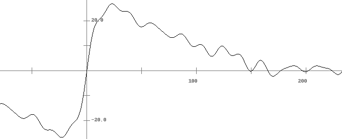
from math import sin

def f(x):
    n = 27
    t = 0
    for i in range(50):
        t += sin(10*x/n)
        n = (n//2) if n%2==0 else 3*n+1
    return t
h Approx 0.1 .4609 0.05 .4387 0.025 .4275 0.0125 .4218
x y 0 0 2 1.414 4 2 6 2.449 8 2.828 10 3.162

Exercises for Chapter 5
correct to within .001 by first using a change of variables. The exact answer is .77976 to 5 significant figures.

(a) Use the substitution u = 1/x and apply the midpoint method to the resulting integral.
(b) Use the substitution u = 1/√x and apply the midpoint method to the resulting integral.
(c) Use the substitution u = 1/√x and apply the trapezoid method to the resulting integral.
(d) Use the substitution u = 1/x2 and apply the trapezoid method to the resulting integral.
from tkinter import *
from math import *

def trap(f, a, b, n):
    dx = (b-a)/n
    return dx/2*(f(a)+f(b) + 2*sum(f(a+i*dx) for i in range(1,n)))

def plot():
    t = -10
    oldx = func1(t) * 100 + 200
    oldy = func2(t) * -100 + 200
    while t < 10:
        t += .01
        x = func1(t) * 100 + 200
        y = func2(t) * -100 + 200
        canvas.create_line(oldx, oldy, x, y)
        oldx = x
        oldy = y

func1 = lambda t:cos(t)
func2 = lambda t:sin(t)

root = Tk()
canvas = Canvas(width=400, height=400, bg='white')
canvas.grid(row=0, column=0)
plot()
cbrt function below to do cube roots as raising things to the 1/3 power won't work quite right. [Hints: The nonzero roots are near ± 1.87. Use FTC Part 1 to find f′(x).]
def cbrt(x):
    return x**(1/3) if x>=0 else -(-x)**(1/3)

def trap(f, a, b, n):
    dx = (b-a)/n
    return dx/2*(f(a)+f(b) + 2*sum(f(a+i*dx) for i in range(1,n)))
- Modify the provided Python Monte Carlo program provided earlier to write a Python function that estimates ∫ba∫dc f(x, y) dy dx.
- Use it to estimate ∫52∫73 (x2+y2) dy dx. The exact answer is 472.
There is also an iterative midpoint rule that is developed from the midpoint rule in a similar way that the iterative trapezoid rule is developed from the trapezoid rule. The major difference is that where the iterative trapezoid rule cuts the step size h in half at every step, the iterative midpoint rule has to cut the step size into a third (i.e. hn+1 = hn/3).
- Using an example, explain why cutting the step size in half won't work for the extended midpoint rule, but cutting it into a third does work.
- Modify the included Python code provided earlier for the iterative trapezoid rule to implement the iterative midpoint rule. Be careful: several things have to change.
Exercises for Chapter 6
- Consider the IVP y′ = t sin y, y(0) = 1, t ∈ [0, 4]. Estimate a solution to it by hand with the following methods (using a calculator to help with the computations):
- Euler's Method by hand with h = 2
- Explicit trapezoid method by hand with h = 2
- Midpoint Method by hand with h = 2
- RK4 by hand with h = 4
- Consider the IVP y′ = –5y, y(1) = .25, t ∈ [1, 2]. Estimate a solution to it by hand with the following methods (using a calculator to help with the computations):
- Use the backward (implicit) Euler method with h = 1 to approximate y(2).
- Use the predictor-corrector method using Euler's method as the predictor and the backward Euler method as the corrector with h = 1 to approximate y(2).
- Use the Adams Bashforth 2-step method with h = 1 to approximate y(3), given y(1) = .25 and y(2) = .002.
- Consider the IVP y′ = 2ty, y(2) = 1, t ∈ [2, 6]. Estimate a solution to it by hand with the following methods (using a calculator to help with the computations):
- Euler's method with h = 2
- The midpoint method with h = 4
- RK4 with h = 4
- AB2 with h = 2 using y(4) as the Euler's method estimate of y(4) (so you know y(2) and y(4) and are using them to find y(6) with the AB2 formula)
- Backward (implicit) Euler with h = 4
- The Euler/Backward Euler predictor corrector with h = 4
- Consider the system x′ = 2y+t, y′ = xy, x(0) = 2, y(0) = –1, t ∈ [0, 4]. Estimate a solution to it by hand with the following methods (using a calculator to help with the computations):
- Euler's method
- Explicit trapezoid method (be careful)
- Rewrite y‴+2y″+ sin(y′) + y = ex as a system of first order equations.
- Write y(4) = ty″+3y′–ety as a system of first order ODEs.
- Use Euler's method with step size h = 2 to estimate the solution to x′ = 2y+t, y′ = xy, x(0) = 5, y(0) = 3, t ∈ [0, 2].
- Use Euler's method with step size h = 2 to estimate the solution to x′ = 2yt, y′ = y–x–2t, x(0) = 3, y(0) = 4, t ∈ [0, 2].
- Use Euler's Method with step size h = 2 to estimate the solution to y″ = ty2, y(4) = 3, y′(4) = 5, t ∈ [4, 6].
- Use Euler's method with h = 1 to solve y″–t(y′)2+ sin(y) = 0, y(2) = 3, y′(2) = 5, t ∈ [2, 3].
- Below shows the result of running the leapfrog method with step sizes h/2 through h/16. Complete the next two columns of the table that would be produced by extrapolating these values.
Step size Estimate First Extrapolation Second Extrapolation h/2 3.4641 — — h/4 3.2594 — h/6 3.2064 h/8 3.1839 h/10 3.1720 h/12 3.1648 h/14 3.1600 h/16 3.1567 - For the ODE extrapolation method, suppose we are solving the IVP y′ = f(t, y), y(2) = y0, t ∈ [2, 3] with h = .1.
- For the first subinterval, the 5th leapfrog step will evaluate the function at which values of t?
- Show below are the first few entries in the extrapolation table. Fill in the missing entries.

- What is a differential equation? Why do we need all these methods for numerically solving them?
- What is an IVP?
- Rewrite the integration problem ∫52 ex2 dx as an initial value (differential equation) problem.
- Arrange the following numerical ODE methods in increasing order of accuracy: Euler's method, RK4, Midpoint method
- Explain, using the ideas of slope fields, how the midpoint method is an improvement on Euler's method.
- Explain, using the ideas of slope fields, where all the parts of the RK4 method come from.
- Explain geometrically how Euler's method works and describe how the formula for Euler's method relates to your geometrical explanation.
- Explain, using the ideas of slope fields, how the midpoint method is an improvement on Euler's method.
- Explain why global error for a numerical ODE method is more than just a sum of local errors.
- How a does predictor-corrector method avoid the root-finding step in the implicit method that is part of the predictor-corrector pair?
- Explain the ideas behind how the implicit (backward) Euler method works and how we can develop a predictor-corrector method based on it.
- Give one benefit that the Adams Bashforth 2-step method has over the midpoint method.
- Give one advantage multistep methods have over single-step methods and one advantage that single-step methods have over multistep methods.
- Implicit methods are mostly used for stiff equations, but they can be used for non-stiff equations. But usually explicit methods are preferred in that case. Why?
- Roughly, what makes “stiff” ODEs difficult to solve numerically, and what type of numerical methods are recommended for solving them?
- One adaptive step-size ODE method we talked about starts by computing the Euler and Midpoint estimates for the same h value.
- What value does it compute from there?
- How does it use that value to decide on a new h?
- True or False (give a reason) — The RK4 method can be used to estimate ∫10 3√1+x2 dx.
- In your own words, describe the basic ideas of the extrapolation method for solving differential equations that we covered in these notes. Be sure to discuss the similarities to and differences from Romberg integration.
- Suppose we want to use the extrapolation method to estimate the solution to an IVP on the interval [0, 3] with a step size of h = 1. To do this, we will end up calling the leapfrog method precisely how many times?
- Consider the following IVP:

- Use Euler's method with h = 2. Do this by hand (with a calculator to help with the computations). Show all your work.
- Use a spreadsheet to implement Euler's method to numerically solve the IVP using h = .1.
- The exact solution is y = 3e sin t. Use a spreadsheet to plot your solutions from parts (a) and (b) on the same graph as the exact solution. Shown below is what your plot should look like.

- Consider the IVP y′ = t sin y, y(0) = 1, t ∈ [0, 4]. Estimate a solution to it using the following:
- Euler's Method by spreadsheet with h = .01
- Explicit trapezoid method by spreadsheet with h = .01
- Midpoint Method by spreadsheet with h = .01
- RK4 by spreadsheet with h = .01
- For the system x′ = 2y+t, y′ = xy, x(0) = 5, y(0) = 3, t ∈ [0, 2], use the following to estimate a solution:
- Euler's method by spreadsheet with h = .01
- Midpoint method by spreadsheet with h = .01
- For the IVP y″ = ty2, y(4) = 3, y′(4) = 5, t ∈ [4, 6], use the following to estimate a solution:
- Euler's method by spreadsheet with h = .01
- Midpoint method by spreadsheet with h = .01
- Here is the Adams-Bashforth four-step method:
 Here fi = f(ti, yi). It requires four initial points to get started. You can use the midpoint rule or RK4 to generate them.
Modify the Adams-Bashforth two-step program provided earlier to implement the four-step method.
Here fi = f(ti, yi). It requires four initial points to get started. You can use the midpoint rule or RK4 to generate them.
Modify the Adams-Bashforth two-step program provided earlier to implement the four-step method.
- In Section 6.8 there is a predictor-correct method using the Adams-Bashforth four-step method along with the Adams-Moulton three-step method. Implement this method in Python.
- Modify the backward Euler program given earlier to implement the implicit trapezoid method.
Bibliography
In writing this, I relied especially on Numerical Analysis by Timothy Sauer, which I have taught from a couple of times. For practical advice, I relied on Numerical Recipes by Press, Teukolsky, Vetterling, and Flannery. From time to time, I also consulted A Friendly Introduction to Numerical Analysis by Brian Bradie and Numerical Methods by Faires and Burden. I also read through a number of Wikipedia articles and online lecture notes from a variety of places.