Notes for Probability
Counting
Probabilities of events can often be done by counting. A simple example is the probability that a roll of a die comes out to an odd number. There are three odd possibilities (1, 3, and 5) and six total possibilities, so the probability of rolling an odd number is 3/6. Interesting probabilities can be calculated in this way using more sophisticated types of counting, so we will study counting for a while.
The multiplication rule
Consider the following question:
An ice cream parlor has types of cones, 35 flavors, and 5 types of toppings. Assuming you get one cone, one scoop of ice cream, and one topping, how many orders are possible?
The answer is 3 × 35 × 5 = 525 orders. For each of the 3 cones, there are 35 different flavors of ice cream, so there are 3 × 35 = 105 possible cone/flavor combinations. Then for each of those 105 combinations, there are 5 different toppings, leading to 105 × 5 = 525 possible orders.
Here is another question:
How many possible strings of 2 capital letters are there?
The answer is 26 × 26 = 576. The possible strings include AA, AB, …, AZ then BA, BB, …, BZ, all the way down to ZA, ZB, …, ZZ. That is, 26 possible strings starting with A, 26 with B, etc., and 26 possible starting values. So there are 26 × 26 or 262 possibilities.
One visual technique that helps with a problems like this is to draw some slots for the possibilities:
 If instead of 2 capital letters, we have 6 capital letters, there would be 266 possibilities. We might draw the slots for the letters like below:
 These examples lead us to the following useful rule:
Multiplication Rule: If there are x possibilities for one thing and y possibilities for another, then there are x × y ways of combining both possibilities.
It's a simple rule, but it is an important building block in more sophisticated counting problems. Here are a few more examples:
- A password can consist of capital and lowercase letters, the digits 0 through 9, and any of 32 different special characters. How many 6-character passwords are possible?
There are 26+26+10+32 different possibilities for each character, or 94 possibilities in total. With 6 characters, there are thus 946 = 689, 869, 781, 056. The slot diagram is shown below:
 Is this a lot of passwords? Not really. Good password-cracking programs that make use of a computer's graphics processing unit can scan through tens of billions of passwords per second. So they would be able to crack a 6-character password in under a minute.
- The old system for phone numbers was as follows: All possible phone numbers were of the form ABC-DEF-GHIJ, where A, D, and F could be any digits from 2 through 9, B could be either a 0 or a 1, and the others could be any digit. How many phone numbers were possible under this system?
The slot diagram helps make things clear:
 So there are 8 × 2 × 10 × 8 × 10 × 8 × 104 = 1, 024, 000, 000 phone numbers. If 50 million new phone numbers were issued each year (after reusing old ones), we can see that we would run out of numbers after about 20 years.
- How many times does the print statement below get executed?
for i = 1 to 1000
    for j = 1 to 200
        for k = 1 to 50
            print "hi"
The answer is 1000 × 200 × 50 = 10, 000, 000 times. - A website has a customizable brochure, where there are 66 possible checkboxes. Checking or unchecking one of them determines if certain information will be or not be included in the brochure. How many brochures are possible?
There are two possibilities for each checkbox (checked or unchecked), and 66 possible checkboxes. See the figure below:
 So there are 266 ≈ 7.3 × 10¹⁹ possible brochures.
- A combination lock consists of a code of 3 numbers, where each number can run from 1 through 39. How long would it take to break into the lock just by trying all the possibilities?
There are 393 = 59, 319 possibilities in total. Assuming 10 seconds to check a combination, we are looking at about 164 hours.
Multiplication rule with no repeats
We know that there are 266 6-character strings of capital letters. What if repeats are not allowed? In that case, while there are still 26 possibilities for the first character, there are only 25 possibilities for the second letter since we can't reuse the first letter. There are 24 possibilities for the next letter, 23 for the next, etc. See the diagram below:
 There are thus 26 × 25 × 24 × 23 × 22 × 21 = 165, 765, 600 possibilities in total.
This type of argument can be used in other situations when counting things without repetition. In particular, it is used to count how many ways there are to rearrange things.
Rearranging things
Suppose we want to know how many ways there are to rearrange the letters ABCDEFG. There are 7 possibilities for what to make the first letter, then once that is used, there are 6 possibilities for the second, 5 for the third, etc. See the figure below:
 So there are 7! possibilities in total. In general we have to following:
There are n! ways to rearrange a set of n different objects. Such a rearrangement is called a permutation.
Here are a couple of examples:
- You and 4 friends play a game where order matters. To be fair, you want to play all the possible orderings of the game. How many such orderings are there?
There are 5 people, so there are 5! = 120 ways of rearranging them.
- You want to take a trip through 6 cities. There is a flight from each city to each other one. How many possible trip orders could you take?
There are 6! = 720 orders in which you could visit the cities.
- A rather silly sorting algorithm, called Bogosort, involves randomly rearranging the elements in an array and checking to see if they are in order. It stops when the array is sorted. How many steps would it take to sort an array of 1000 elements?
While it could in theory take only one step, on average it will take around 1000! steps, since there are 1000! ways to rearrange the elements of the array and only one of those corresponds to a sorted array.**Note that 1000! is a particularly large number, being about 2500 digits long.
Rearrangements with repeats
Suppose we want to know how many ways there are to rearrange a collection of items with repeats. For example, how many ways are there to rearrange the letters of the string AAB?
Suppose for a moment that the A's were different, say aAB instead of AAB. Then the 6 possible rearrangements would be as follows:
aAB, AaB,
aBA, ABa,
BAa, BaA
If we turn the lowercase a back into an uppercase A, then the first row's rearrangements both correspond to AAB, the second row's correspond to ABA, and the third row's correspond to BAA. For each of these three classes, there are 2! ways to rearrange the A's if they were different. From this we get that there are 6!2! ways to rearrange AAB. In general, we have the following:
The number of rearrangements of a collection of n items where item 1 occurs m1 times, item 2 occurs m2 times, etc. is(where k is the number of distinct items).
I usually just think of this rule as the “Mississippi rule,” based on the first problem below.
- How many ways are there to rearrange the letters in the word MISSISSIPPI?
There are 11 letters in MISSISSIPPI, consisting of 1 M, 4 I's, 4 S's, and 2 P's, so the number of rearrangements is

- Suppose we want to know how many possible ways 10 rolls of a die could occur in which we end up with exactly 4 ones, 2 twos, and 4 sixes.
This is equivalent to rearranging the string 1111226666. There are 10!4! · 2! · 4! = 3150 ways in total.
Subsets
Here is a question: How many subsets of {A, B, C, D, E, F} are there in total?
To answer this, when we create a subset, we can think of going through the elements one at a time, choosing whether or not to include the element in the subset. For instance, for the subset {A, D, F}, we include A, leave out B and C, include D, leave out E, and include F. We can encode this as the string 100101, with a 1 meaning “include” and a 0 meaning “leave out,” like in the figure below:
     A B C D E F
     1 0 0 1 0 1
     A     D   F
Each subset corresponds to such a string of zeros and ones, and vice-versa. There are 26 such strings, and so there are 26 possible subsets.
In general, we have the following:
There are 2n possible subsets of an n-element set.
Now let's consider a related question: How many 2-element subsets of {A, B, C, D, E, F} are there?
As described above, two-element subsets of {A, B, C, D, E, F} correspond to strings of zeros and ones with exactly 2 ones and 4 zeros. So we just want to know how many ways there are to rearrange the string 110000. There are 6!2!4! = 15 such ways.
A similar argument works in general to show that there are n!k!(n–k)! k-element subsets of an n-element subset. This expression is important enough to have its own notation, (nk). It is called a binomial coefficient. In general, we have
 The rightmost expression comes because a lot of terms cancel out from the factorials. It is usually the easiest one to use for computing binomial coefficients. In that expression, there will be the same number of terms in the numerator and denominator, with the terms in the denominator starting at k and working their way down, while the terms in the numerator start at n and work their way down.
To summarize, we have the following:
The number of k-element subsets of an n-element set is (nk).
As an example, the number of 3-element subsets of a 7-element set is
 As another example, the number of 4-element subsets of a 10-element set is

There are a lot of counting problems that involve binomial coefficients. Here are a few examples:
- How many 5-card hands are possible from an ordinary deck of 52 cards?
There are (525) ≈ 2.6 million hands.
- How many ways are there to choose a group of 3 students from a class of 20?
There are (203) = 1140 possible groups.
In general, (nk) tells us how many ways there are to pick a group of k different things from a group of n things, where the order of the picked things doesn't matter.
Multinomial coefficients
The last problem of the previous section showed that there are (203) = 20!3!17! ways to choose a group of 3 students from a class of 20. Suppose we want to from multiple groups from that group of 20—say a group of 3 students that comprise the homework committee and a group of 4 students that comprise the exams committee, where no one is allowed to served on two committees at once. We can think labeling all students as either H, E, or N, for whether they are on the homework committee, exams committee, or neither. So we have a string of 20 letters with 3 H's, 4 E's, and 13 N's. The number of ways we can rearrange this string is the same as the number of ways to break students up into these committees. This is the Mississippi problem, and the answer is 20!3!4!13!.
Notice the similarity in this answer to the answer (203) = 20!3!17! to the problem from the previous section. A natural way to represent the new answer, 20!3!4!13!, is as (203, 4). This is called a multinomial coefficient. It's not as widely used as the binomial coefficient, but it is still nice to know about.
A few rules for working with binomial coefficients
Here are a few quick rules for working with binomial coefficients:
- (n0) = 1 and (nn) = 1.
That is, there is one 0-element subset of a set (the empty set) and one n-element subset of an n-element set (the set itself).
- (nk) = (nn–k)
This is useful computationally. For instance, (2017) is the same as (203).
- Binomial coefficients correspond to entries in Pascal's triangle. Here are the first few rows.
                            1
                         1     1
                      1     2     1
                   1     3     3     1
                1     4     6     4     1
             1     5    10    10     5     1
          1     6    15    20    15     6     1
The top entry is (00). The two entries below it are (10) and (11). In general, the entry in row n, column k (starting counting at 0) is (nk). - Binomial coefficients show up in the very useful binomial formula:
 The easy way to get the coefficients is to use Pascal's triangle. Here are a few examples of the formula:
 Here is a little more complicated example:

Combinations with repeats
When counting things, there are often two main considerations: if repeats allowed and if order matters. There are four cases in total, summarized in the table below. We have so far talked about three of these cases, but not yet about the bottom left case.
| repeats allowed | repeats not allowed | |
| order matters | nk | n(n–1) ··· (n–k+1) |
| order doesn't matter | (n+k–1n–1) | (nk) |
The top left entry is the basic multiplication rule. The top right entry is the multiplication rule with repeats. This is actually a type of permutation, and people sometimes use the notation nPk or P(n, k) or the formula n!(n–k)! for it. The bottom right entry is for subsets or combinations. Sometimes people use the notation nCk or C(n, k) for it.
The bottom left is for combinations with repeats, also known as multisets. For instance, maybe we want to know how many ways there are to rearrange the letters A, B, C, D, and E, where things like AAB, ABA, and BAA are all considered the same. The trick people use to count this is sometimes called “stars and bars”. For this problem, imagine having bins for the letters A, B, C, D, and E, where we put tokens into various bins to represent the multisets. For instance, the AAA multiset corresponds to putting 3 tokens into the A bin and none anywhere else. Since we're looking at 3-letter combinations, we always have 3 tokens to distribute into the various bins. Show below are a few examples using stars to represent the tokens. Bins are separated by bars. The “stars and bars” column below represents the distribution of tokens into bins, with the bars representing separators between bins.

Each combination of letters corresponds to a unique sequence of stars and bars. In this case, there are 3 stars and 4 bars, so there are 7 total characters in each star-bar sequence, so by the Mississippi problem, there are 7!3!4! = (73) such sequences and hence that many combinations of the letters A, B, C, D, and E with repeats allowed.
In general if we want k-element combinations from a set of n items with repeats allowed, the formula is (n–1+kk). This is because there are n–1 bars and k stars. Alternately, this is equivalent to (n–1+kn–1).
Here are a few examples:
- Suppose we want to distribute 10 identical pieces of candy to 7 people. How many ways are there to do this in total?
For instance, maybe person A gets 4 pieces, B gets 3, C gets 3, and everyone else gets nothing. We can write this as the multiset AAAABBBCCC. The set we are choosing from has n = 7 elements, and we are choosing mulitsets of k = 10 items, so the formula gives (10–1+710) = (1610).
- How many solutions to w+x+y+z = 10 are there where the four variables are all nonnegative integers?
Think about it as a multiset problem from the set {W, X, Y, Z} where we are choosing 10-element multisets. A combination like WWWXXYYYYZ corresponds to the solution w = 3, x = 2, y = 4, z = 1. The set we are choosing from has n = 4 elements, and we are choosing combinations of size k = 10, so the formula gives (4–1+1010) = (1310).
- How many times does the print statement run in the code below?
for i = 1 to 9
    for j = 1 to i
        for k = 1 to j
            print('hello')
The first time something is printed, we have i = 1, j = 1, and k = 1. Let's write these i, j, and k values in shorthand as 111. The next time we get 211. After that, we get 221, 222, 311, 321, 322, 331, 332, 333… until finally we get to 999. We can see this is actually generating combinations with repeats of k = 3 items from the set {1, 2, 3, 4, 5, 6, 7, 8, 9} of n = 9 items, so the formula gives (9+3–13) = (113).
Addition rule
Counting problems involving the word “or” usually involve some form of addition. Consider the following very simple question: How many cards in a standard deck are queens or kings? There are 4 queens and 4 kings, so there are 4+4 = 8 in total. We have the following rule:
Addition Rule: If there are x possibilities for A, y possibilities for B, and no way that both things could simultaneously occur, then there are x+y ways that A or B could occur.
Here are some examples:
- What is the probability a three-letter string of capital letters start with A or B?
If we want to use the addition rule for this problem, note that One way to approach this is to note that there are 262 three-letter strings that start with an A and there are 262 that start with B, so there are 262 + 262 that start with A or B.
- Problems containing the words “at least” or “at most” can often be done with the addition rule. For instance, how many 8-character strings of zeros and ones contain at least 6 zeros? The phrase “at least 6 zeros” here means our string could have 6, 7, or 8 zeros. So we add up the number of strings with exactly 6 zeros, the number with exactly 7, and the number with exactly 8.
To get how many contain exactly 6 zeros, think of it this way: There are 8 slots, and 6 of them must be zeros. There are (86) = 28 such ways to do this. Similarly, there are (87) = 8 strings with exactly 7 zeros. And there is 1 (or (88)) strings with 8 zeros.
So there are 28+8+1 = 37 strings with at least 6 zeros.
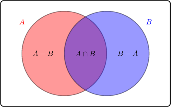
The simple question we started this section out with asked how many cards in a standard deck are queens or kings. What if we change it to ask how many are queens or diamonds? There are 4 queens and 13 diamonds, but the answer is not 17. One of the cards in the deck is the queen of diamonds, which gets double-counted. So there are actually 4+13–1 = 16 cards that are queens or diamonds. In general, we have the following rule:
General addition rule: If there are x possibilities for A, y possibilities for B, and z possibilities where both occur, then there are x+y–z ways that A or B could occur.
An alternate approach to the above rule is to turn the question into an “or” question with no overlap. For instance, to count how many queens or diamonds are in a deck, we can approach it as counting how many cards are queens but not diamonds, how many are diamonds but not queens, and how many are both queens and diamonds. That gives us 12+3+1 = 16 as our answer.
In terms of set notation, we could write the general addition rule as
 And we could write this alternate approach as
 A Venn diagram helps make these formulas clearer:
Here are some examples of the rule:
- How many integers between 1 and 1000 are divisible by 2 or 3?
Every second integer is divisible by 2, so there are 500 integers divisible by 2. Every third integer is divisible by 3, so there are ⌊1000/3⌋ = 333 integers divisible by 3. However, multiples of 6 are double-counted as they are divisible by both 2 and 3, so we have to subtract them off. There are ⌊1000/6⌋ = 166 of them. So in total, 500+333–166 = 667 integers are divisible by 2 or 3.
- How many three-character strings of capital letters start or end with a vowel (A, E, I, O, or U)?
We can add up the ones that start with a vowel and the ones that end with a vowel, but words that both start and end with a vowel are double-counted. To fix this problem, we have to subtract them from the total. See the slot diagram below:

In total, there are 5 × 262 + 5 × 262 – 52 × 26 = 6110 ways.
Alternatively, we could approach the problem as shown in the slot diagram below:
 That is, we break things up into three disjoint possibilities: things that start but don't end with a vowel, things that end but don't start with a vowel, and things that both start and end with a variable. This gives 5 × 26 × 21 + 21 × 26 × 5 + 5 × 26 × 21 = 6110.
Negation rule
Another simple question: How many cards in a standard deck are not twos? There are 52 cards and 4 twos, so there are 48 cards that are not twos. In general, we have
Negation rule: To compute the number of ways that A can't happen, count the number of ways it can happen and subtract from the total number of possibilities.
Using set notation, we could write this as |AC| = |U|–|A|, where U is the universal set (which changes depending on the problem). Here are a couple of examples:
- How many integers from 1 to 1000 are not divisible by 2 or 3?
In the previous section, we found that 667 of those integers are divisible by 2 or 3, so there are 1000–667 = 333 that are not divisible by 2 or 3.
- How many strings of 6 capital letters have at least one vowel?
The phrase “at least one vowel” means would could have 1, 2, 3, 4, 5, or 6 vowels. That could get tedious to compute. But the complement of having at least one vowel is having no vowels at all. So we can approach this problem by finding how many strings of 6 capital letters there are (which is 266) and subtracting how many contain no vowels (which is 216). So our answer is 266–216 = 223, 149, 655.
Cards and counting
Let's look at some questions about cards. A standard deck of cards contains 52 cards. Those 52 cards are broken into four suits: clubs, diamonds, spades, and hearts, with 13 cards in each suit. In each suit there is a 2, 3, 4, 5, 6, 7, 8, 9,10, jack, queen, king, and ace.
- How many 5-card hands are there?
When you're dealt a card hand, it is a subset of 5 different cards from the deck, so there are (525) ≈ 2.6 million possible hands.
We can use this value to turn all of the following questions into questions about probability. For instance, a royal flush is a hand where the five cards are 10, jack, queen, king, and ace, all of the same suit. There are exactly 4 ways to get a royal flush, one for each suit. So the probability of a royal flush is 4/(525), which is 1 in every 649,740 hands.
- How many 5-card hands are flushes, where all five cards are the same suit?
There are 13 cards in each of the 4 suits: diamonds, hearts, clubs, and spades. So there are (135) hands that contain only hearts. Likewise there are (135) hands that contain only hearts, and similarly for the other two suits. So overall, there are (135) + (135) + (135) + (135) possible flush hands.
We can also look at this via the multiplication rule as 4 · (135), where we first choose the suit (one of four choices) and then choose 5 cards from that suit.
- How many hands are straight flushes, where all five cards are from the same suit and are in order (like 3,4,5,6,7 or 7,8,9,10,jack)?
There are 4 choices for each suit and 10 types of straights (starting from ace,2,3,4,5 running up through 10,jack,queen,king,ace), so there are 4 · 10 = 40 straight flushes.
- How many five-card hands are straights? A straight is where the cards are in order.
As above, there are 10 types of straights. Each of the five cards can be any of the four suits, so there are 45 ways those suits can come up. In total, there are 10 · 45 possible suits.
- How many five-card hands are full houses?
A full house is where three of the cards of one kind and two of another, like three jacks and two kings or three 7s and two aces.
There are 13 choices for the first group of three cards and 12 choices for the second group. For that group of three, there are 4 suits to choose those 3 cards from, so there are (43) ways. In the group of two, there are (42) ways to pick those two cards. So all told, it's 13 · (43) · 12 · (42).
- How many five-card hands are four-a-kind, where four of the cards have the same value?
There are 13 choices for what that four-of-a-kind is, and we have to take all of the cards from that kind. That leaves 48 possibilities for the last card, so there are 13 · 48 ways to get four-of-a-kind.
- How many five-card hands are three-a-kind, where three of the cards have the same value. When people say three-of-a-kind, they usually mean it's not also a four-of-a-kind or a full house. So we're looking at three cards that are of the same kind and two other cards that are different from the three-of-a-kind and different from each other.
There are 13 choices for the three-of-a-kind's value. Since we are only taking 3 of the 4 cards of the that value, there are (43) ways to choose those. The fourth card can't have the same value as the three-of-a-kind, so there are 48 cards to choose from for that. The fifth card has to be different in value from the first four, so there are 44 possibilities for this. For the fourth and fifth cards, to multiply 48 · 44 isn't quite correct because that would be the case for when order matters. But in card hands, order doesn't matter, so we have to divide by 2!, which is the number of ways to rearrange the fourth and fifth cards. Putting everything together, the answer is
 Another way to look at the fourth and fifth cards is as (122) · 42, where we need to pick two different values, and for each there are 4 choices for the suit.
Example problems
Here are some example problems.
- This problem is about lining up 8 people.
- How many different ways are there to line them up?
This is a basic permutation. There are 8! ways.
- How many ways are there to line them up if two of them (say A and B) must always be next to each other?
The trick is to treat A and B as if there were a single person. So now there are essentially 7 people to line up, so there are 7! ways to do this. However, within the A/B group, there are 2! ways they could be lined up (as AB or BA), so there 7! · 2 is the final answer to the problem.
- Suppose the 8 people consist of 3 boys and 5 girls, and the rule is that there must be a boy in the second position of the line and a girl in the fourth position.
For the second position there are 3 choices and for the sixth there are 5 choices. That leaves 6 choices for the first slot, 5 for the third, and 4, 3, 2, and 1, respectively for the remaining positions. So there are 5 · 3 · 6! ways in total.
- How many different ways are there to line them up?
- Suppose we want to make a committee of 3 people from a group of 8. However, 2 people, A and B, refuse to be in a group together. How many committees are possible?
Break this up into three disjoint pieces: committees containing A but not B, committees containing B but not A, and committees containing neither. If we want A and not B, that means that after choosing A for the group, there are 2 slots left, and 6 people to choose them from, so there are (62) possibilities. The same reasoning shows there are (62) committees with B and not A. There are (63) groups that contain neither A nor B, since we are picking 3 people from 8–2 = 6 people. Using the addition rule to get
 An alternate approach that there are (83) total committees possible, and (61) = 6 of them are bad committees that contain both A and B, so the good ones are (83)–6.
- Suppose we want to make a committee of 3 people from a group of 8, specifying one of them to be the committee president. How many ways are there to do this?
There are 8 people to choose as president and then (72) ways to pick the other two members, so the final answer is 8 · (72).
- Suppose we have a class of 20 students and we want to assign a presentation to 7 of them, with no one being assigned more than one presentation. How many ways are there to do this?
This is actually a subset problem in disguise. We are essentially picking a group of 7 students from a group of 20, so the answer is (207).
- Suppose we have a class of 20 students. We want to assign a presentation to 7 of them, a homework to 5 of them, and an exam to 3 of them, with no one having more than one thing to do. How many ways are there to do this?
One approach is to first assign the presentations. There are (207) ways to do this. Then assign the homework to 5 of the remaining students. There are (135) ways to do this. Finally, assign the exam to 3 of whoever is left, which is (83) ways. Multiply all this together to get (207)(135)(83).
An alternate approach is to think of this as a multinomial coefficient or Mississippi problem, where we have (207, 5, 3) = 20!7!5!3!.
- Being able to tell when order matters and when it doesn't can sometimes be tricky. For instance, suppose we have 4 people A, B, C, and D, that we want to break into two groups of 2, suppose one of the groups will meet in person and the other virtually. How many ways are there to do this? The answer is (42) · (22) = 6.
What if we change the question so we just want to pair off the 4 people into two groups of 2, with nothing special distinguishing the groups. Now the answer is (42) · (22)/2!=3. Why is this different from the other case? In the first case, having A and B be in the in-person group and C and D be in the virtual group is different from having C and D be in the in-person group and A and B be in the virtual group. In the second case, assigning A and B to one group means the other group would have C and D, but there is nothing special distinguishing the groups, so if we first assign A and B to a group and then assigned C and D to the other, that wouldn't be any different than first assigning C and D and then assigning A and B.
In the case where order doesn't matter, we have to divide by 2!, which is the number of ways to order the groups. That is, the breakdown (AB, CD) could also occur in the order (CD, AB), which is the same.
- Counting problems can be very subtle, and it's easy to make a mistake where we end up overcounting things. For example, suppose we want to know how many 5-card hands contain at least one card of every suit. One way to approach the problem would be to first pick one card of each of the four suits to ensure we have at least one in each suit, and then pick two other cards from what is left. Since there are 13 choices in each suit, this gives 134(482).
However, this is not correct. It overcounts things. Consider the hand that consists of all four aces along with a king of spades and a king of clubs. That hand is counted once by thinking of the first four cards that are picked (the 134 part of the answer) as being the aces and the two kings being the remaining two cards (the (482) part of the answer). But that hand is also counted again by thinking of the first four cards as being the ace of hearts, ace of diamonds, king of spades and king of clubs, with the other two cards being the remaining two aces.
To catch yourself from overcounting things, look at all the terms of your answer and see the same item could be counted in two different ways by assigning its parts to different terms.
One correct solution to this problem is to think of it in terms of assigning suits. Specifically, since there are five cards, with at least one of each suit, the hand will consist of three suits that have one card each and one other suit that has two cards. There are four choices for the suit with two cards and (132) cards from that suit. From the other suits, there are 13 cards to choose from, so the answer is 4 · 133 · (132).
Basics of Probability
Definitions
Defining probability can be tricky. Here is a common approach: Start with the concept of an experiment, which is, roughly speaking, where you observe something that is random or uncertain. That experiment has various possible outcomes. The set of all possible outcomes of that experiment is called the sample space. An event is a subset of the sample space. A probability of an event is a real number we assign to that event. We denote the probability of event A by P(A). Probabilities must satisfy certain properties known as Kolmogorov's axioms of probability. Assuming S is the sample space A, here are the three axioms:
- P(A) ≥ 0 for every event A.
- P(S) = 1.
- if A1, A2, A3, … are disjoint events, then P(A1 ∪ A2 ∪ A3 ∪ …) = P(A1)+P(A2)+P(A3)+….
Let's use an example to illustrate the vocabulary. Suppose we roll an ordinary six-sided die. Here is what all the terms correspond to in this example:
- Experiment: rolling the die
- Outcomes: what can happen when rolling the die, specifically what value is rolled
- Sample space: {1, 2, 3, 4, 5, 6}
- Events: subsets of the sample space, like {2} corresponding to rolling a 2, or {2, 4, 6} corresponding to rolling an even number
- Probabilities: For a die, each outcome has probability 1/6. So for example, we have P({2}) = 1/6 and P({2, 4, 6}) = 1/6+1/6+1/6 = 1/2.
All the rules of probability can be derived from Kolmogorov's axioms. This isn't a theoretical course, so we won't do this, but it's worth looking at it a little bit. In particular, let's show that P(AC) = 1 – P(A). In real world terms, this is saying that the probability that A doesn't happen is 1 minus the probability it does. To prove this, start with the fact that A ∪ AC = S. The sets A and AC are disjoint, so by the third axiom, we have P(A ∪ AC) = P(A) + P(AC). By the second axiom, P(S) = 1, so we have P(A)+P(AC) = P(A ∪ AC) = P(S) = 1. Subtract to get P(AC) = 1 – P(A), as desired. As a bonus, this shows probabilities must always be less than or equal to 1 because if P(A) > 1, then P(AC) < 0, which breaks the first axiom.
Notation and useful rules
Below is some common notation. Assume A and B are events. Thinking of events as sets, set notation can be used to describe common probabilities. This is very similar to a counting rule we saw earlier. A Venn diagram of overlapping sets A and B can be helpful in seeing why this rule is true. It can be proved without too much work from the axioms, but we will not do that here. An important special case is if A and B are mutually exclusive. In that case P(AB) = 0 and the rule becomes P(A ∪ B) = P(A)+P(B).
Another way to do the probability of A or B is shown below:
 Again, this is very similar to a rule we saw for counting. Venn diagrams help for seeing why it is true, and it follows directly from basic set theory and the third axiom.
 The probability that A happens and B doesn't is P(A–B) or P(ABC) . It is given by

It helps to think of one of the dice as colored red and the other blue. There are 62 = 36 outcomes in total. We can systematically list them as (1, 1), (1, 2), (1, 3), …, (6, 6), where the first entry in each ordered pair is the value of the red die and the second is the value of the blue die. The table below groups all the outcomes by sum. Those outcomes are given in a shorthand notation with something like (3, 1) being shortened to 31. Each of the 36 outcomes is equally likely, so we can use this to get probabilities of each of the sums.
| total | outcomes | prob. | percent |
| 2 | 11 | 1/36 | 2.8% |
| 3 | 12, 21 | 2/36 | 5.6% |
| 4 | 13, 22, 31 | 3/36 | 8.3% |
| 5 | 14, 23, 32, 41 | 4/36 | 11.1% |
| 6 | 15, 24, 33, 42, 51 | 5/36 | 13.9% |
| 7 | 16, 25, 34, 43, 52, 61 | 6/36 | 16.7% |
| 8 | 26, 35, 44, 53, 62 | 5/36 | 13.9% |
| 9 | 36, 45, 54, 63 | 4/36 | 11.1% |
| 10 | 46, 55, 64 | 3/36 | 8.3% |
| 11 | 56, 65 | 2/36 | 5.6% |
| 12 | 66 | 1/36 | 2.8% |
Conditional probabilities
Suppose we have a jar with 7 red and 3 blue marbles. The probability of picking a red marble is 7/10. Let's say we pick a marble, see that it is red, set it aside, and pick another marble. What is the probability that marble is red too? After removing the one red marble, there are 6 red and 3 blue marbles in the jar, so the probability that second marble is red is 6/9. This probability is an example of a conditional probability. The “conditional” part of the name comes from the fact that we want the probability of one event given that another event has already happened (the condition). The notation for this is P(B | A), which is read as the probability of “B given A”. It's the probability that B happens given that A has already happened. Below is the formula used to compute it:
 The idea is that since we are given that A happens, we are restricting ourselves to just those outcomes that are part of A. This the denominator. The numerator is which of those outcomes also are part of B. Here is a concrete example: Suppose there are 1000 students at a school with 200 taking math, and 50 taking both math and history. Given a student is taking math, what is the probability they are also taking history? It's 50/200, the fraction of those math students taking history over the total number of math students. Using the formula, A is the event that a student is taking math and B is the event they are taking history, and we have


 For instance, going back to the marble problem from the beginning of the section, there are 7 red and 3 blue marbles. Suppose we pick a marble, set it aside, and pick another. What is the probability both are red? Let A be the event that the first is red and let B be the event that the second is red. We are looking for P(AB), the probability that both picks come out red. We have P(A) = 710, and P(B| A) = 69 since if the first is red, then there are 6 red and 9 total marbles left. So using the formula, we have P(AB) = P(A)P(B | A) = 710 · 69.
For P(ABCD) the formula would be P(A)P(B | A)P(C| AB)P(D | ABC), and the formula can naturally be extended to larger intersections.
 This is the exact same thing we would get doing the problem by picking the marbles one at a time and setting them aside. For other problems of this sort, remember that picking things all at once is the same as picking them one at a time and setting them aside.
Independence
Sometimes P(B | A) turns out to equal P(B). That is, the fact that A occurs has no effect the probability of B occurring. A common example is a coin flip. If A is the event that the first flip comes out heads and B is the event that the second comes out heads, then P(B|A) = 1/2, which is the same as P(B). That first flip has no effect on the second. This is part of the concept of independence.If A and B are independent, P(B| A) = P(AB)P(A) = P(A)P(B)P(A) = P(B). Similarly, P(A| B) = P(A). That is, if either A or B happens, it has no effect on the chances of the other occurring. Note that the definition naturally extends to more events. For instance, events A, B, and C are independent provided P(ABC) = P(A)P(B)P(C). In general, for however many events we have, if they are independent, then the probability that they all happen is gotten by multiplying their individual probabilities.
Here are a few examples:
- If we flip a coin twice, what is the probability both flips are heads?
Coin flips are independent of each other, each with probability 12 of heads, so the probability they are both heads is 12 · 12 = 14.
- If we roll a die 10 times, what is the probability all 10 rolls are twos?
The multiplication rule for independence works regardless of how many events we have, so we multiply 16 by itself 10 times to get (16)10, which is around a 1 in 60 million chance.
- Suppose the weather forecast for a certain area calls for a 20% chance of afternoon thunderstorms every day during the summer. If you are there on vacation for a week, what is the probability there is a storm there every day, assuming independence?
The answer is (.20)7, which is .0000128, or 1 in 78125.
Trying to account for dependence can get very tricky, so if the dependence between events is pretty small, people usually ignore it and assume the events are independent. It makes the probability much easier to calculate and usually doesn't have a large effect on the answer.
However, sometimes assuming independence can lead to incorrect results. In 2010 in the Washington, DC area, there were three very large snowstorms. A news report at the time said that snowstorms of that size happen only about once in every hundred years, so the probability of three of them in a single year would be (1100)3, which is 1 in a million. This would be true if the storms were independent, but they were not. Once an area gets into a particular weather patter, big storms become more likely, and it stays that way until the weather pattern shifts. So the fact that a storm occurred actually means the area may have been in a weather pattern favoring storms, meaning the probability of another storm is higher than it otherwise would be. In other words, independence is a bad assumption.
However, suppose we have a jar with 700 reds and 300 blues. Let's repeat the same question. If we pick two like above, the probability both are red is 7001000 · 699999, which is .4897. This not too far off from 7001000 · 7001000 = .49. So, assuming independence in this case wouldn't be so bad. For large enough populations, this is what is usually done. For instance, 11% of people worldwide are left-handed. If we pick 2 people at random, what is the probability they are both left-handed? If we treat them as independent, the answer is (.11)2, which is 1.21%. However, they are technically not independent since the first person being left-handed reduces the number of left-handed and total people when calculating the probability for the second person, just like when we remove a marble from a jar. However, doing the problem that way and assuming a world population of 8 billion gives an answer of 1.2099999988%. The small difference between this and 1.21% is not worth the extra effort, especially considering there are bigger sources of error possible in problems like this.
The terms with replacement and without replacement are used to describe scenarios where items are put back after being picked or are set aside. Events are independent when items are picked with replacement, but they are not independent when picked without replacement. However, if the number of items is large enough and we are not picking too many items, then as we saw above, there is not much difference in the answers whether things are replaced or not. In this case, we can usually get a good approximate answer by pretending things are done with replacement.
On the other hand, P(AB) = P(A)P(B) for independent events. The events don't have any effect on each other, and it is possible for both of them to happen, unlike with mutually exclusive events.
Example problems
In this section we will use the rules from the previous sections to answer some probability questions.
- If you roll an ordinary die 20 times, what's the probability you get no fours?
The probability of a four is 16, so the probability of not getting a four is 56. Dice rolls are independent, so we can multiply the probabilities to get (56)20, which is about 2.6%. If you've ever played a dice game and needed a specific value, you know it can sometimes take quite a while to get it.
- Suppose someone can correctly pick the winner of an NCAA tournament game 95% of the time. What is the probability they correctly pick the winners of all of the games? There are 64 teams in the tournament.
First we need to know how many games there are. One way is that there are 32 games in the first round, 16 in the second, then 8, 4, 2, and 1, which sums to 63. The clever way to do this is that one team wins the whole tournament and every other team has exactly one loss, so there must be 64–1 = 63 total games played.
Assuming independence, the probability the person picks all the games right is (.95)63, which is around 3.9%. You never hear of people picking all the games right, so probably no one can pick games with 95% accuracy.
- A multiple choice test has 10 questions, with 4 answer choices for each. What is the probability a person randomly guessing gets all 10 right?
Since we are randomly guessing, each guess is independent and we have a 1/4 chance of guessing any given question correctly. So the probability of a getting them all right is (14)10, which is around a one in a million chance.
- Suppose we pick 3 cards from a deck at once. What is the probability they are all aces?
There are 4 aces and 52 cards in a deck. We can treat this like the marble problem and get 452 · 351 · 250. Remember that picking cards all at once is equivalent to picking them one at a time and setting them aside after each pick. We could also do the problem as (43)/(523). It's about a 1 in 5525 chance.
- A class has 5 juniors and 10 seniors. A professor randomly calls on 4 different students. What is the probability they are all seniors?
Since the professor is calling on different students, the events are not independent, and we can solve it via 1015 · 914 · 813712 or via (104)/(154).
- A jar has 4 red, 5 blue, and 6 green marbles. You reach in and pick 2. What is the probability both are the same color?
They could be both red, both blue, or both green. These are mutually exclusive events, so we add their probabilities to get 415 · 314 + 515 · 414 + 615 · 514.
- If you flip a coin 5 times, what is the probability all 5 flips come out the same?
This is similar to the last one. There are two ways they could all come out the same: either as all heads or as all tails. The answer is (12)5 + (12)5.
At least one problems
A common probability problem is to ask for the probability of at least one occurrence of an event. For example, suppose there is a 20% chance of rain for each of the next 7 days. Assuming independence, what is the probability it rains at least once?The event that it rains at least once includes the possibilities that it rains one time, twice, three times, etc. While we could compute the probabilities of each of those possibilities separately and add them, there is a better way. The complement of the event that it rains at least once is that it doesn't rain at all. So we'll compute the probability that it doesn't rain at all, and subtract that from 1. We get 1–(.80)7, which is about 79%.
In general, we have the following rule: To get the probability of at least one occurrence of something, do 1 minus the probability of no occurrences.
Here is another example: Suppose we have an alarm clock that works correctly 99% of the time and malfunctions 1% of the time. That is, 1 in every 100 days, even if you set it right, it still doesn't go off. If we have four of these alarm clocks, what is the probability at least one works correctly?
We do this as 1 minus the probability that none of them work, which is 1 – (.01)4 = .99999999, a very high probability. This is important. If we have several components that are all unreliable, if we take enough of them, we can get a pretty reliable result, assuming independence. Of course, if things are not independent, then this doesn't necessarily work. For instance, if all four alarms are plugged into the same outlet and the power goes out, then we're in trouble.
More examples
- In Texas Hold'em, you are dealt 2 cards. There are also 5 community cards, and players try to make the best 5-card hand they can between their cards and the community cards. The first 3 community cards are put out and then the fourth and fifth are put out after that.
- Suppose you are dealt 2 clubs and the first 3 community cards contain 1 club. What is the your probability of making flush? Assume you don't know what anyone else's cards are.
For a flush, you need the remaining two community cards to be clubs. There are 47 cards remaining in the deck and 10 of them are clubs (remember that we don't know what anyone else's cards are, so theoretically any 2 of the remaining 47 cards can come out as the other community cards). So the probability is 1047 · 946, which is around 4.2%.
- Suppose the scenario is like in part (a) except that the first 3 community cards contain 2 clubs, what is the probability of a flush now?
Now you can get a flush if the fourth, fifth, or both come out as clubs. We could do those three probabilities separately, but it's quicker to just do 1 minus the probability that neither are clubs. There are 38 non-clubs in the deck, and we get 1–3847 · 3746, which is about 35%.
- Suppose you are dealt 2 clubs and the first 3 community cards contain 1 club. What is the your probability of making flush? Assume you don't know what anyone else's cards are.
- Suppose you flip a coin 5 times. What are the probabilities of getting 0, 1, 2, 3, 4, and 5 heads?
Think about the outcomes as strings of 5 characters, each either H or T, such as HHHHH or HTHTH. There are 25 = 32 of them in total, and there are (5k) of them that contain k copies of the letter H since that is how many ways there are to locate k copies of the letter H in 5 spaces. So the probability of exactly k heads is (5k)/32. The values for k = 0 to 5 are roughly 3%, 16%, 32%, 32%, 16% and 3%, respectively.
- If you are in a room with 183 other people. What is the probability someone has the same birthday as you? Ignore the possibility of a leap-day birthday.
This is an at least one problem. We can treat it as 1 minus the probability that no one has the same birthday as you, which is 1–(364365)183, or about 39%.
- If we put 10 numbers in a box and pick all of them out one after another without replacement, what is the probability they come out in order from 1 to 10?
There are 10! ways to rearrange them, and only one of those is in order, so it's 1/10!.
- If we randomly rearrange the letters A, B, C, D, E, there is a 1/5! chance they come out in order. What if we arrange those letters around a circle? What is the probability they come out in order?
The probability changes from lining them up in a line. In a line, there is a clear start and end, but not in a circle. Any of the 5 spots can serve as the start in a circle. So there are only 4! ways to rearrange the letters on a circle.
- Suppose we pick 3 random capital letters with replacement. What is the probability we get no repeats?
One approach is that there are 263 ways to pick 3 capital letters, and there are 26 · 25 · 24 ways to pick 3 capital letters with no repeats, so the probability is 26 · 25 · 24263.
Another way to approach the problem is that the first letter can be anything and after that there is a 2526 chance that the second letter doesn't repeat with the first, and a 2426 chance that the third doesn't repeat with either of the first two. So overall, we could write it as 2626 · 2526 · 2426, which agrees with our other way of doing things.
This is a special case of a more general problem: Picking k objects from a set of n objects with replacement. If k ≤ n, then the probability of no repeats is n(n–1)(n–2)…(n–k+1)nk or n!/(n–k)!nk. If k > n, the formula breaks down.
- Earlier, we counted how many ways there are to get various types of 5-card hands. Dividing those by the (525) total card hands gives us probabilities. For instance, a flush has probability 4 · (135)/(525), a four-of-a-kind has probability 13 · 48/(525) and a full house has probability 13 · (43) · 12 · (42)/(525).
We can talk about similar types of problems for rolling 5 dice. The answers will be somewhat different since the cards can't repeat in a hand, but dice values can. As we saw with the two-dice probabilities we looked at earlier, it's helpful to think of the dice each being a different color.
- What's the probability of rolling five-of-a-kind, where all five dice are equal?
One approach is there is a (16)5 probability of rolling all ones. This is the same for each of the values. Adding up the probabilities of these 6 mutually exclusive events gives 6 · (16)5 = (16)4. We could also approach it from a counting perspective, thinking of it as there being 6 possible five-of-a-kinds and 65 total ways the dice could come out, so we get 6/65 = 1/64. One other approach is to go die-by-die. For the first die, it could be anything, but then each of the remaining 4 dice must match that first die's value, each with a 1/6 probability of doing so, so it's (16)4, which corresponds to a 1 in 1296 chance.
- What's the probability of rolling four-of-a-kind, where four of the dice are equal and the other is different?
There are 6 possibilities for the value that comes out four times. And there are (54) choices of which 4 of the 5 dice have that value. There are 5 possibilities for the remaining die, so overall the probability is (6 · (54) · 5)/65. This is about 1.9% or about 1 in every 52 rolls.
- What's the probability of rolling a full house, where there are 3 of one value and 2 of another, like 3,3,3,2,2 or 5,5,5,1,1?
There are 6 choices for the first value and (53) ways to pick which 3 dice have that value. There are then 5 choices for the second value, and there is no choice left for which dice those are. So the overall probability is 6 · (53) · 5/65, which is about 3.9% or about 1 in every 26 rolls.
For the (53) part, we could also think about it in terms of the number of ways to rearrange the values . For instance, 33322 could be rearranged as 33223, 32233, 22333, and several other ways, thinking in terms of the Mississippi problem.
- What's the probability of rolling five-of-a-kind, where all five dice are equal?
- Two people take turns rolling a die until a six comes up. What is the probability the first player wins?
There is a 16 probability they win right away. Their next opportunity to win on roll 3. For us to get to this point, the first 2 rolls must not have been sixes and now the winning roll is a six. So the probability for this is (56)216. The next opportunity for them to win is on roll 5. For this to happen, we must have 4 rolls without sixes followed by a six, giving us the probability (56)416. In theory, this game could go on indefinitely, and we end up with the following infinite sum:

We can rewrite this in sigma notation as ∑k = 0^∞ 16(2536)n. This is in the form of a geometric series. You might remember the formula for geometric series: ∑n = 0^∞ rn = 11–r provided |r| < 1. Here we have r = 2536, so we end up with 16 · 11–25/36, which simplifies to 611, or about 54%. So the first player has a slight edge.
A clever way to approach the problem is as follows: Let x be the probability the first player wins. They have a 16 chance of winning on their first roll. Their next chance of winning is on the third roll, and because the rolls are independent, their probability of winning once they get to that point is still x. However, it took two non-sixes to get to that point, so we can say x = 16 + (56)2x. Solve for x to get x = 611.
- Roll two dice until the sum is either 5 or 7. What is the probability we get a sum of 5 before we get a sum of 7?
This is similar to the last problem. First, note that there are 36 outcomes from rolling two dice. There are 4 of them that give a sum of 5, there are 6 of them that give a sum of 7, and the remaining 26 outcomes give a sum of neither. Using a geometric series approach like the last problem, we get the following:
 Alternatively, using the same clever approach as in the previous problem, we could write the equation x = 436+2636x and solve to get x = 25.
- How many possible states are there that a Rubik's Cube can be in?
There are 8 corner pieces, 12 edge pieces, and 6 center pieces. The centers can't move independently of the other pieces. Any corner piece can be moved to any another corner piece's location, so there are 8! ways the corner pieces can be located (think of it as lining up the 8 pieces in 8 locations). Each corner piece has 3 visible sides, so there are 38 ways in total the corners can be oriented.
The edge pieces work similarly. There are 12! ways to locate them, and each edge has 2 visible faces, so there are 212 ways the edges can be oriented. Putting this together gives 8! · 38 · 12! · 212.
However, there is an additional trick. Not every one of these states is physically possible. In particular, when we rotate the corners, once 7 of the 8 corners are positioned, the orientation of the last corner is fixed, so we have to divide out by 3. For a similar reason involving the edges, we have to divide out by 2. And there is one other complication that has to do with so-called even and odd permutations which means there is one additional factor of 2 to divide by. So the total number of possible states is
 If we were to disassemble and reassemble the cube, those couple of complications don't arise and there are 8! · 38 · 12! · 212. This differs from the earlier answer by a factor of 12, which tells us that if we disassemble the cube and randomly put it back together, there is a 1 in 12 chance that it will be solvable.
Finally, if we peal off all 54 stickers from the pieces, there are 54!/(24 · (9!)6) ways to put them back. This is because there are 54 individual stickers, so there are 54! ways to put them back. However, there are 9 stickers in each of 6 colors, so using the Mississippi problem, we get 54!/(9!)6 ways to arrange the stickers. This still overcounts things. Think about a cube that is solved with the green side facing up. If we flip it over, that's really not a different state, just a different way of positioning the cube. Our current answer has the same problem. There are 24 different ways to position the cube. Specifically, there are 6 possible faces that can be on top, and then 4 ways we could rotate the other faces. So putting it all together, we get 54!/(24 · (9!)6) ≈ 4.2 × 1036. This is much larger than the number of states on a Rubik's cube. If you randomly rearrange the stickers, the probability is nearly 0 that it will be solvable.
The birthday problem
How many people do there have to be in a room for there to be a 50/50 chance some pair of people in the room have the same birthday?
This is the famous birthday problem. Note that this is different from an earlier problem we asked about birthdays. In that problem, we were interested in someone having the same birthday as us. Even with 183 people in the room, the probability is under 50%. But in this problem, we just want some pair of people in the room to have the same birthday, and there are lots of possible pairs, which will bring the number down considerably from 183.
The problem is famous because the answer is so surprisingly low. To figure out the answer, let's treat it as an at least one problem. We want the probability that there is at least one shared birthday. So we'll do 1 minus the probability that there are no repeated birthdays. This is like the letter-choosing we did a few problems back. If there are k people in the room, the probability of at least one repeat is (ignoring leap-year birthdays)
 We can use this formula to put together a spreadsheet or computer program to look at probabilities for various values of k. See below for some values:
| # in room | Probability of two people sharing a birthday |
| 5 | 2.7% |
| 10 | 11.7% |
| 20 | 41.1% |
| 23 | 50.7% |
| 30 | 70.6% |
| 40 | 89.1% |
| 50 | 97.0% |
| 60 | 99.4% |
| 70 | 99.9% |
| 80 | 99.99% |
| 90 | 99.999% |
| 100 | 99.99997% |
With a little math, we can get a formula that we can use to solve the probability formula approximately for k. Specifically, starting with the probability formula, rewrite it in a clever way as in the second line below, and then use the fact that ex ≈ 1+x.

Invert this to get the number of people needed for there to be a probability p of a repeat:
 There is nothing special about birthdays here. We can use a similar formula for other situations where we are interested in the probability of a repeat when picking from a set of n items:
 And, the most commonly used rule of thumb is that after √n things are generated, repeats are fairly likely (when p is around .4, the formula above simplifies to √n).
As an example, if we are generating random numbers from 1 to a million, repeats start becoming likely after around √1000000 = 1000 numbers are generated.
As another example, recall that there are (525) ≈ 2.6 million card hands. If you are dealt a hand right now, the probability that you will ever see that exact hand again is small. However, the probability that at some point in your card-playing life you get dealt a hand that you had been dealt at some point in the past is actually pretty high. By the birthday problem, repeats become likely after around √\binom{52{5}}, which is around 1600 hands. If you play 10,000 hands in your life, the formula says the probability of a repeated hand is approximately 1–e–100002/(2 · \binom{52{5})} ≈ .99999999586.
Important probability rules
Inclusion-exclusion
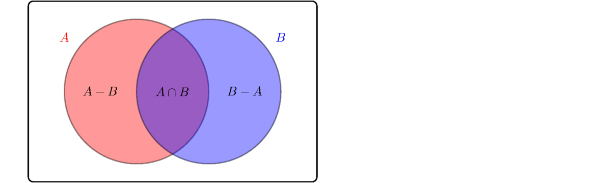
The rule P(A ∪ B) = P(A)+P(B)–P(AB) is very similar to the counting rule |A ∪ B| = |A|+|B|–|A ∩ B| we saw much earlier. The Venn diagram below helps us see why it must be true: if we take we want the stuff in A or B, we can get it by adding together the stuff in A and the stuff in B, but then the stuff in the overlap gets counted twice, so we correct by subtracting that off.
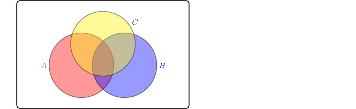
The idea extends to unions of more terms. For instance,


 There are 5! total outcomes, and we want the complement of what we just found, so the final probability is 1–76/5! ≈ .378.
It's not too hard to generalize this idea. For n people, the inclusion-exclusion for the number of outcomes in the union would give
 Here, the k variable stands for the size of the sets, which is the size of the overlap. The (–1)k+1 term alternates positive and negative, the (nk) term comes from the number of sets of each size from 1 to n, and the (n–k)! term comes from there being k people that get their own hats back and n–k that don't, and those are the ones that are rearranged. If we write out (nk) as n!/(k!(n–k)!), we can cancel the (n–k)! terms to simplify the sum into the following:
 To get a probability, we divide by n! and negate to get
 We can cancel out the n! terms, and move the negative inside the sum to get
 Finally, (–1)k+2 is the same as (–1)k and note that since 1 is the same as (–1)0/0!, we can reindex things to make it just a single sum, like this:
 You may remember from a calculus class that the power series of ex is 1+x+x2/2!+x3/3!+…. The series above is the power series for e–1 or 1/e, cut off after n terms. Thus, as n gets larger, the probability approaches 1/e ≈ 0.367879.
We'll do this with the counting version of inclusion-exclusion and divide by 6! (total ways to arrange the names) at the end to convert it to a probability. We'll also approach this via the negation, counting the ways for there to be three or more names that end up in order.
Let A be the event that the first three names are in order, let B be the event that names 2, 3, and 4 are in order, let C be the event that names 3, 4, 5 are in order, and let D be the event that the last three names are in order. The number of outcomes in of each of these events is (63) · 3! = 120 since there are (63) ways to pick 3 of the 6 names to be the ones in order and 3! ways to rearrange the other 3 names.
However, there is overlap between each of these sets. In particular, we need to look at the events AB, AC, AD, BC, BD, and CD. Event AB would mean that names 1, 2, 3 as well as 2, 3, 4 are in order. In other words, the first 4 names are in order. Similarly to how it worked for 3 names in order, the number of outcomes for 4 in order is (64) · 2! = 30. The event AC is similar, but in this case, we get 5 things in order, so it's (65) · 1! = 6. The event AD is a little different. This is where 1, 2, 3 are in order and 4, 5, 6 are in order. Here there are (63) = 20 ways to pick the first 3 names and once those names are picked, there is only 1 way to pick the last 3 names. So there are 20 outcomes in AC. Events BC and CD have 30 outcomes each, similar to AB, and event BD has 6, similar to AC.
Next, we have to look at the three-way overlaps—ABC, ABD, ACD, and BCD. Event ABC corresponds the first 5 being in order, which we already saw has 6 outcomes. Events ABD and ACD correspond to all 6 being in order, which is 1 outcome each. And event BCD corresponds to the last 5 being in order, which is 6 outcomes. Finally, the four-way overlap ABCD corresponds to everyone being in order, which is one outcome. So we have

So there are 371 total outcomes where 3 or more of the names are in order. So we negate and divide by 6! to get the probability that no more than 2 of the names are in order. This is 1–3716! ≈ .48.
Law of total probability
If A and B are events, then by basic set theory, B = AB ∪ ACB. See below.
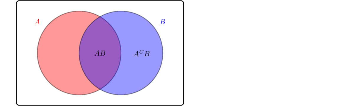
Since AB and ACB are disjoint, we have P(B) = P(AB)+P(ACB) by Kolmogorov's third axiom. The definition of conditional probability tells us P(AB) = P(B|A)P(A) and P(ACB) = P(B|AC)P(AC). Plugging these into the previous equation gives
 This is a very useful rule called the law of total probability. The idea is that if we want the probability of B, and B is affected by some other event A, then we consider two cases: A happens or A doesn't. We compute the conditional probability of B is each case and weight those probabilities by the probabilities of A and AC, respectively. People often refer to this approach as
“conditioning on A”.
This is a very useful rule called the law of total probability. The idea is that if we want the probability of B, and B is affected by some other event A, then we consider two cases: A happens or A doesn't. We compute the conditional probability of B is each case and weight those probabilities by the probabilities of A and AC, respectively. People often refer to this approach as
“conditioning on A”.
There is a more general version of the rule that applies if A1, A2, …, An are disjoint events whose union equals the entire sample space. The sets Ai are said to partition the sample space. None of the events have any outcomes in common and every possible outcome is in exactly one of them.
In this case, the total probability formula is

Here are a few example problems.
- Suppose a school buys its chairs from two distributors, X and Y. They get 80% of their chairs from X and the rest from Y. Further, assume 5% of X's chairs are defective, and 15% of Y's are. If we pick a random one of the school's chairs, what is the probability it is defective?
Let A be the event that the chair is one of X's chairs, and let B be the event that the chair is defective. We want P(B). The law of total probability lets us compute P(B) by looking at chairs from X and Y separately. Specifically, P(B|A) = .05, the probability that a chair is defective given it is from X; P(A) = .8, the probability a chair is one of X's; P(B|AC) = .15, the probability that a chair is defective given it is from Y; and P(AC) = .2, the probability a chair is one of Y's. Putting this together gives
 This is a lot like a weighted average, where we weight the two types of chairs' probabilities of being defective by the percentage of chairs of that type. The tree diagram below might be helpful in seeing how this works. For it, we'll just pick a number of chairs, say 100, though any value works. At the end, we see that in total 7 of the 100 chairs are defective.

- There are three jars of marbles. Jar 1 contains 7 red and 3 blue. Jar 2 contains 2 red and 18 blue. Jar 3 contains 30 red and 70 blue. If I pick a single marble from a random jar, what is the probability it is red?
We'll use the total probability rule with three terms, one for each jar. Specifically, A1, A2, and A3 will be the events that jars 1, 2, or 3, respectively, are chosen, and B is the event that a red it chosen. Assuming the jars are equally likely to be chosen, we have

- Suppose we pick 2 cards from a deck at once. What is the probability the first is an ace and the second is a diamond?
The trick here is that the first card could be a diamond or it could not, which both lead to different probabilities for the second card being a diamond. We will use the law of total probability, conditioning on whether the first card is the ace of diamonds or not. Let A1 be the event that the first card is the ace of diamonds, let A2 be the event that the first card is an ace other than the ace of diamonds, and let A3 be the event that the first card is not an ace. Let B be the event that the second card is a diamond and the first is an ace. We have

- Consider the following dice game: The goal is to get 2 sixes. You get 2 rolls to do so, and if you get 1 six on the first roll, you can set it aside and just roll the other die for the second roll. What is your probability of winning?
Let's condition on the number of sixes we get on our first roll: 0, 1, or 2. Specifically, let A0, A1, and A2 represent those events, and let B be the event that we win the game. Here is the computation:

Looking at the first term, the one for getting no sixes on the first roll, P(A0) = 2536, which is (56)2, coming from a 56 chance for each die to not be a six. The other part of that term, P(B|A0) = 136, comes from needing both dice to be sixes, which is (16)2. The other terms work similarly. Note that the probability of exactly one six on the first roll can be gotten by subtracting the probabilities of 0 and 2 sixes from 1.
This is a simplified version of the game Yahtzee, where you roll 5 dice and one of the goals is to get all 5 of the dice to be the same. You get 3 tries to do so, and you can store dice from roll to roll, like in this problem. Computing the probability of a Yahtzee can be done using only things we've already learned, but involves going through quite a few cases, so we will not do that here.
- Suppose there are three dice. Two of them are fair dice, and the other is weighted so that a six comes out 80% of the time. If we pick a random one of those dice, what is the probability we roll a six?
Let A1, A2, and A3 be the events that the first, second, and third dice, respectively, were chosen, and assume the third die is the weighted one. Let B be the event that we roll a six. Then

- Suppose we pull the ace of spades out of an ordinary deck of cards. We shuffle the remaining cards and deal out 25 cards. We put the ace of spades in with those 25 cards and shuffle all 26 of them. If we pick a random card from these 26, what is the probability it is an ace?
We condition on whether the card we pick is the ace of spaces or not. Let A be the event that the card we picked is the ace of spaces and let B be the event that we picked an ace. We have
 Going through this term by term, P(A) is 126 since we know the ace of spaces is one of those 26 cards, and P(B|A) = 1 since if the ace of spaces was what we picked, then it is certainly an ace. Next, P(AC), the probability of not picking the ace of spaces, is 2526. Finally, P(B|AC), the probability of picking an ace given that we didn't pick the ace of spades, is 351. This is because each card other than the ace of spaces has an equal chance of ending up in the collection of 26 cards, so we are essentially looking at the probability of picking one of the 3 aces out of the 51 cards left after removing the ace of spades.
Bayes' Theorem
Bayes' Theorem is one of the most useful and arguably the most famous theorem in probability, giving rise to a whole approach to probability and statistics called the Bayesian approach.
The idea is this: Suppose we need P(A|B), but it seems hard to compute. However, maybe P(B|A) and P(B|AC) are easy to compute. Bayes' theorem gives a way to use these to get P(A|B).
To get the formula, start with the definitions P(B|A) = P(AB)/P(A) and P(A|B) = P(AB)/P(B). Solve the first for P(AB) and plug into the second to get P(A|B) = P(A)P(B|A)/P(B). Then plug in the total probability formula P(B) = P(B|A)P(A) + P(B|AC)P(AC) to get Bayes' theorem

A more general version of Bayes' theorem works if we have events A1, A2, …, An that partition the sample space. The rule is

- In the section on total probability, there was a problem about a school that buys its chairs from two distributors, X and Y. They get 80% of their chairs from X and the rest from Y. Assume 5% of X's chairs are defective, and 15% of Y's are. We had early asked if a random chair is chosen, what is the probability it is defective. With Bayes' theorem, we can now answer a different question: if one of the school's chairs is defective, what is the probability it is a chair from X?
There are two competing influences here: one the one hand, Y chairs are more likely to be defective, and on the other hand, most of the chairs at the school are X chairs. Let's let A be the event that the chair is an X chair and let B be the event that the chair is defective. We want P(A|B). Bayes' theorem allows us to find this in terms of P(B|A) and P(B|AC), which are things we know, namely the probabilities that each distributors chairs are defective. Bayes' theorem gives
 We can also see where this comes from using the tree diagram below. In that diagram, we assume there are 100 chairs (the number we choose doesn't matter). This tells us that on average there should be 4 defective X chairs and 3 defective Y chairs, so the probability a defective chair is an X chair is 4/7. Bayes' theorem works similarly, just working with the raw probabilities instead of converting into numbers of chairs.

- Suppose there are three dice. Two of them are fair dice, and the other is weighted so that a six comes out 80% of the time. If you pick a random one of those dice and roll a six, what is the probability the die you picked was the weighted one?
This problem is also similar to one with did when looking at total probability. In that problem, we just wanted the probability of a six. Now we want something more interesting. Let A1, A2, and A3 be the events that the first, second, and third dice, respectively, were chosen, with the third die being the weighted one. Let B be the event that a six was rolled. Bayes' theorem lets us answer the tricky probability P(A3|B) in terms of things we know:

- Bayes' Theorem is important in something known as the base rate fallacy. A well-known example of it involves tests for diseases. Suppose we have a test that has 99% accuracy. By this we mean that if you have the disease, there is a 99% chance the test will come out positive for the disease, and if you don't have the disease, there is a 99% chance the test will come out negative, saying you don't have the disease. If you take the test and get a positive result, what is the probability you actually have the disease?
We don't yet have enough information to answer the problem. The base rate fallacy is that most people would say the answer is 99%, without taking into account the base rate, namely how prevalent the disease is in the population. Let's suppose that 1 in every 500 people has the disease (probability of .002). How does this affect the probability that you have the disease, given you got a positive test?
Let A be the event that you have the disease and let B be the event that you got a positive test. We want P(A|B). We get
 So instead of a 99% probability of having the disease, the actual chance is around 16.6%. Why the difference? Suppose the population is 1,000,000 people. Then there are 2000 people with the disease in that population and 998,000 without. Of those 2000 people with the disease, 99%, or 1980 will get a positive test. Of the 998,000 without the disease, 1% or 9980 will get a positive test. These are false positives. There are many more false positives than true positives, and the number of true positives, 1980, is around 16.6% out of the total positives.
- An answer key was taken from a professor's office. The professor claims to be 60% certain that Person X took the answer key. Person X has blond hair. Then some new camera footage shows that the person that took the answer key has blond hair. How does should this new information change the professor's percent certainty that Person X took it? Note that roughly 20% of people have blond hair.
Let A be the event that Person X took the answer key, and let B be the event that the person who took it had blond hair. Bayes' theorem gives
 Let's look at this term by term. First, P(B|A) is the probability that the person who took it has blond hair given that it was Person X that took it. This is 100% since Person X does have blond hair. Next, P(B|AC) is the probability that the person who took it has blond hair given that it was someone other than person X that took it. Here we have to use the 20% prevalence of blond hair in the overall population. Finally, P(A) and P(AC) are the probabilities that Person X did and did not take it, and we use the professor's prior certainty for these. The result of the calculation tells us that the professor should update their certainty to 88%. This type of Bayesian approach to updating things when new information comes in is used in many fields, especially in statistics.
The Monty Hall problem
This problem comes from the 1970s version of the game show Let's Make a Deal. There was a game where there are three doors. Behind one of them is a prize, usually a car, and behind the other two are fake prizes, usually goats. You pick the door you think has the prize. Then Monty, who knows where the prize is, shows you a door that doesn't have the prize. There are now two doors left, and he asks if you want to switch doors? Should you, shouldn't you, or does it not matter?
When first seeing this, many people say that since there are two doors left, it's 50-50 where the prize is, so it doesn't matter. The reason why the problem is so famous is that the answer is not 50-50. You're actually better off switching. This problem was posed in the Ask Marilyn column that went out to millions of newspaper subscribers in 1990. She correctly answered the question, but then she received thousands of angry letters, some from professional mathematicians, telling her how wrong they thought she was.
To understand why it's better to switch, consider that you have a 1/3 chance of correctly guessing the door right at the start. There is a 2/3 chance that the prize is behind one of the other doors. That never changes. The key fact is that Monty doesn't randomly choose any door to open. He will always open a door different than yours and different from the one that contains the prize. He is essentially collapsing that 2/3 probability onto the other door. So you have a 1/3 chance of winning if you stick with your guess and a 2/3 chance if you switch.
Another way that helps me think about it is to imagine that there are 100 doors instead of 3. You pick a random door to start, and there's a 1/100 chance you've picked right. Then Monty, who knows where the prize is, opens up 98 other doors, leaving just your door and other. Should you switch? Yes. There's a 1/100 chance your door is the right one, a 99/100 chance the prize is behind another door, and Monty was helpful enough to narrow things down for you.
Going back to the 3-door problem, if Monty could randomly open any door, including yours and the one with the prize, then the game would often end before you got a chance to switch. If you did get far enough to switch, then the probability in that case would be 1/2. The key element that makes the Monty Hall problem not be a 1/2 probability is that Monty knows where the prize is and will always eliminate a door that doesn't have the prize.
A tree approach
If you're not convinced yet that you should switch, here is a mathematical argument using a tree diagram. For this diagram, assume that the prize is behind Door 1.
The first branch is for your choice of door. Each choice you make has a 1/3 probability. The second set of branches is for which door Monty opens. In the first case, where you pick Door 1, Monty can open either of Door 2 or Door 3, both equally likely with probability 1/2. For the second case, if you pick Door 2, Monty has to open Door 3 since he can't open Door 1 with the prize behind it. So the probability he opens Door 3 is 1. The third case is similar. To get the probabilities of each of the four outcomes at the ends of the tree, multiply the probabilities. The first two have probability 1/6 and the last two have probability 1/3. Now, since the prize is behind Door 1, if you choose Door 1 and then switch, you lose. The probabilities for both those events are 1/6 + 1/6 = 1/3> If you choose Door 2 and switch, you win. The probability of that is 1/3. Similarly, the probability of winning if you choose Door 3 and switch is 1/3. So overall, there is a 1/3 chance you win if you stick with your initial choice and a 2/3 chance you win if you switch.
A Bayes' theorem approach
For this approach, let's suppose you pick door 1 and Monty opens Door 2. What is the probability the prize is behind Door 3? For i = 1, 2, 3, let Ai be the event that prize is behind Door i. Let B be the event that Monty opens Door 2. We are interested in P(A1|B), the probability that the prize is behind Door 1 given that Monty opens Door 2. Bayes' Theorem lets us flip this around. In particular, it gives
Where do all the values come from? To start, P(A1) = P(A2) = P(A3) = 1/3 since the prize is equally likely to be behind any of the doors. Next, P(B|A1) is the probability that Monty opens Door 2 given that the prize is behind Door 1. This is 1/2 since if the prize is behind Door 1, then he could choose either Door 2 or Door 3. Next, P(B|A2) is the probability that Monty opens Door 2 given that the prize is behind that same door. This is 0 since he always shows you a door that doesn't have the prize, so he can't open this door. Finally, P(B|A3) is the probability Monty opens Door 2 given that the prize is behind Door 3. This is 1 since he can't open Door 3 since it has the prize and he can't open Door 1 since that's your door.
In all, we see you have a 1/3 chance of winning if you stick with the door you initially chose.
A simulation
If you don't trust the math, you could always try playing the game a bunch of times yourself and seeing how often you win if you switch. A computer can simulate playing many times. Here is some code to do that.
from random import choice, randint

count = 0
for i in range(10000):
    prize = randint(1,3)
    guess = randint(1,3)
    opened = choice(list({1,2,3}-set([prize, guess])))
    other = ({1,2,3} - set([guess, opened])).pop()
    if other == prize:
        count += 1

print(count / 10000)
The door is randomly chosen as well as the player's guess. Monty will always open a door that does not contain the prize and is not the player's guess. That's what the opened variable is. The other variable is the other door left after Monty opens one of the doors. That's the door we would switch to. The code uses Python's set data type to make it quick to remove doors from the possible choices.
If you run the code, you'll see that the result varies a bit from run to run, but overall the values are very close to 2/3.
Random variables
A random variable, roughly speaking, is a variable whose value is determined by some random process. Usually random variables are real numbers, though they don't have to be.
Here is an example: Suppose we flip a coin 5 times. One random variable associated with this experiment is the number of heads we get. This variable takes on integer values from 0 to 5. As another example, suppose we roll a die until we get a six. A random variable associated with this experiment is the number of rolls it takes to get that six. This random variable takes on all integer values greater than 0. As a final example, suppose we are looking at the lifetime of a lightbulb. In theory, we could know its exact lifetime if we had precise information about exactly how often it is used, exactly what voltages it deals with over its lifetime, exactly how much tungsten is used in its filament, etc., in practice there is no way to know all of these things, and it's easier to treat it as a random process. In this case, the lifetime of the bulb is the random variable, and it can take on (in theory) any real value greater than or equal to 0.
A random variable where the domain is a discrete**More rigorously, the domain of a discrete random variable is a countable set, one that can be put into a one-to-one correspondence with the natural numbers ℕ. set like ℤ, ℕ, or a subset of them, is called a discrete random variable. A random variable where the domain is a continuous set like ℝ or an interval, is call a continuous random variables.
To get a little more precise, we can define a random variable X as a function whose domain is the sample space of an experiment. The codomain can be any set, though typically it is something like ℕ, ℤ, ℝ, or [0, ∞). We use the notation P(X = a) for the probability that X has the value a.
For the random variable X, the probability distribution function (or pdf) is a function p(x) defined by p(x) = P(X = x). The term probability mass function is also commonly used to mean the same thing. The cumulative distribution function (or cdf) is defined as f(x) = P(X ≤ x).
As an example, consider the experiment where we flip a coin three times. We can write the sample space as S = {HHH, HHT, HTH, HTT, THH, THT, TTH, TTT}. The number of flips that are heads is a random variable X, which is a function from S to {0, 1, 2, 3}. We have P(X = 0) = 1/8, P(X = 1) = 3/8, P(X = 2) = 3/8, and P(X = 3) = 3/8. The pdf is the function p(x) defined by p(0) = 1/8, p(1) = 3/8, p(2) = 3/8, and p(3) = 1/8. A histogram of it is shown below on the left, basically a bar graph showing each of its values.

Shown above on the right is a graph of the cdf, f(x). The cdf is the sum of all the probability values up to a given point. For instance, f(2) is given by
 The cdf defined for all real numbers, but since the random variable we are looking at is only defined for 0, 1, 2, and 3, the only place things will change in the cdf is in that range. Since this is a discrete random variable, the cdf ends up being a piecewise function. For instance, f(2) = 7/8 but also f(2.3) = 7/8 and f(2.888) = 7/8 since the next place the pdf is defined at is 3.
Expected value
Here is a game: Roll a die. If it's a 1, 2, 3, or 4, you win $50. Otherwise, you lose $90. Is this a good game to play repeatedly?
There are two mathematical factors influencing this: (1) You don't win as much when you win as you lose when you lose ($50 versus $90); (2) You're more likely to win than lose (4/6 versus 2/6). How do we consider both of these factors, the money and the probability? We take a weighted average, weighting the money values by our chances of getting them. Specifically, we have
 How do we interpret this number? It is our average winnings per game. If we play a lot of times, we will win some and lose some, and everything will average out to around $3.33 per game. If we play 100 times, our winnings will likely come out around 100 · 3.33 = $333. In theory, we could win every time, but that is highly improbable. It's also improbably that we come out with exactly $333, but it's likely that we'll end up in the ballpark of that value.
What we just computed above is called an expected value. For any discrete random variable X, the expected value (also called the expectation is given by
 where the sum is taken over all possible values of x.
| heads | 0 | 1 | 2 | 3 |
| prob | 1/8 | 1/8 | 1/8 | 1/8 |
 This expected number of heads, 3/2 or 1.5, is the average number of heads we get from doing this experiment many times. Sometimes we'll get no heads, sometimes 1, etc., but the average amount of heads per experiment is 1.5. The expected value calculation is the same as the physics center of mass calculation. The expected value is thus sort of the center of mass of the probability distribution.
| time | 6:57 | 6:58 | 6:59 | 7:00 | 7:01 | 7:02 | 7:03 |
| prob | .01 | .03 | .10 | .52 | .25 | .07 | .02 |

Suppose you try the following strategy: initially bet $1 on red. If a red number comes out, you win $1. If not, go double or nothing—bet $2 on red. If a red comes out, then you net $1 (you win $2 on this try, but you lose $1 on the first). If a red doesn't come out, go double or nothing again, this time betting $4 on red. If a red comes out, you net $1 again ($4 won minus $1 lost on the first try and $2 lost on the second). If you keep losing, keep going double or nothing up to a maximum bet of $8192. If you get to that point, that would be your 14th turn. The odds of losing on all the turns before and on that turn are (20/38)14, and if you lose then, you lose 1+2+4+8+… + 8192 = 16383 dollars. Notice also, that if you win on some turn, then you end up winning just $1. Is this a good betting strategy? What is the expected value?
The random variable essentially boils down to two values –$16383 or +$1, with probabilities (20/38)14 and 1–(20/38)14, respectively. The expected value is therefore
 So as a long-run betting strategy, this won't work too well. If you do this many times, you will win most of the time, and lose once in great while ((20/38)14 corresponds to a probability of about 1 in 8000). That rare loss is such a large loss that it tends to wipe out all of your winnings.
 This sort of thing works in general, namely if we multiply a random variable by a constant a to get a random variable aX, then E[aX] = aE[X]. This follows directly from the formula of expected value by factoring an a out of the sum. The linearity of the summation operation if fact gives us the following useful properties of expected value:
- For any real numbers a and b, E[aX+b] = aE[X] + b.
- If X1, X2, …, Xn are random variables, then E[X1+X2+… Xn] = E[X1] + E[X2] + … E[Xn].
Variance
Consider these two exams. Exam 1 has scores 60, 70, 80, 90, and 100, while Exam 2 has scores 78, 79, 80, 81, 82. Both have an average of 80. But clearly, the two exams behave very differently. So to summarize a set of data, average isn't enough. We need something else that measures how spread out the data is. To make this more about probability, let's suppose in both scenarios that the five exam scores are equally likely, each with probability 1/5. One way to measure the spread would be to look at the differences between each score and the average. For instance, in the first scenario, the differences are –20, –10, 0, 10, and 20, while in the second scenario the differences are –2, –1, 0, 1, 2. We could try something like with expected value and weight those difference by their probabilities and add them all up. The problem with this is that it comes out to 0 in both cases. To fix this, we need to ignore the signs. We could take the absolute values of the differences. That would work pretty well, except that working with absolute values algebraically and with calculus (which we will soon need to do) is a pain. So instead of absolute values, people usually square the differences to get rid of the signs. The sum of the squares of the differences, weighted by their probabilities, is called the variance of the random variable. For a random variable X, it is denoted by Var(X). It is defined as below, where μ = E[X]:
 With a little bit of algebra, one can derive the alternate formula below that can be a little easier to work with in some cases:
 Squaring all the differences means that the units of the variance are different from the units of the original random variable. To undo this, we can take the square root at the end to get what is called the standard deviation. In particular, the standard deviation, or SD(X), is √Var(X).
| heads | 0 | 1 | 2 | 3 |
| prob | 1/8 | 1/8 | 1/8 | 1/8 |
 Using the alternate formula gives
 We can see the alternate formula is a little quicker to calculate here.
As we saw, expected value is the same calculation as center of mass in physics. Variance is the same calculation as moment of inertia.